Introduction
The goal of this MP is to understand and implement Q-learning algorithm for Reinforcement Learning (RL). The MP will use OpenAI gym library to simulate an RL environment for a taxi dispatch problem as shown in the figure below.
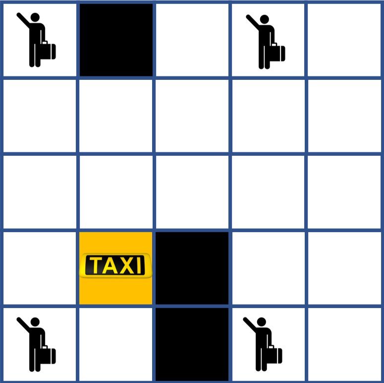
navigation and decision-making task in which an agent (Yellow) drives around a 5×5 grid with a number of pickup and dropoff points, and areas (Black) to be avoided.
RL problems are modeled as a Markov Decision Processes (MDP). An MDP \(M\) is a 5-Tuple as follows:
$$M = (\mathcal{S}, \mathcal{A}, \mathcal{P}, \mathcal{R}, S_0)$$
where \(\mathcal{S}\) is the set of states; \(\mathcal{A}\) is the set actions; \(S_0\subseteq \mathcal{S}\) is the set of initial states; \(\mathcal{P}\) is the (unknown) transition probability matrix of the agent; \(\mathcal{R}: \mathcal{S} \times \mathcal{A} \rightarrow \mathbb{R}_{\geq 0}\) is the reward function.
RL computes a policy \(\pi: \mathcal{S} \rightarrow \mathcal{A}\) such that the following cumulative cost function is minimized:
$$\pi^* := arg\max_{\pi} \mathbb{E} \left[ \sum_{t=0}^{\infty} \gamma^t r(s_t, a_t) | s_0 \sim S_0, a_t \sim \pi(s_t) \right] $$
In this MP, you are going to be implementing the Q-learning Algorithm for computing an optimal policy.
Installation and Environment Setup
You are going to implement this MP in Python using Jupyter notebook.
For installation instructions with Jupyter Notebook, follow the instructions provided in MP1.
After installing Jupyter Notebook, clone the following gitlab repository for the MP using the following command:
git clone https://gitlab.engr.illinois.edu/GolfCar/mp4-release
cd mp4-release
jupyter notebook
Taxi Environment
In the taxi environment, you have a Taxi as depicted by the Yellow block in the environment schematic draw below. The black blocks are to be avoided and the agent has to find the optimal path to pick-up and drop off all the passengers without incurring any penalties (ex: colliding with the black regions).
Two components of the state is the row and column of the current location of the taxi. Next, we need information about the current passengers riding in the taxi. Since there are four passengers, this state could either be \(\{passenger_1, passenger_2, passenger_3, passenger_4, empty\}\). Now, we need to figure out where the passenger needs to go. That gives us our last state component, which indicates the destination of the taxi. Thus, to put all this state information together, we have:
$$state = (rows, cols, passenger\_index, destination\_index)$$
The set of actions A ={N,S,E,W, U, D}, the first four elements correspond to moving one block north (N), south (S), east (E) and west (W), and the last two elements represent picking up (U) and dropping off (D) passengers.
The remaining two of them are either picking up or dropping of passengers if they are at a given location.
In RL problems, the probability transition matrix P is unknown. So, we are not going to be mention it here (however, it would be a good exercise to try to come up with a candidate transition model on your own).
The reward function is provided by the Gym developers and is defined as follows. Every normal time step with no collisions incurs a cost of -1 point. Every illegal action (e.g., an in-correct pickup and drop off) costs -10 points and correct pick-up and drop-off is worth +20 points.
Q-learning Algorithm
Q-learning is a popular method for learning RL policies. Q-learning was first proposed as an alternative to the value-Iteration and policy iteration algorithms you first learned in class.
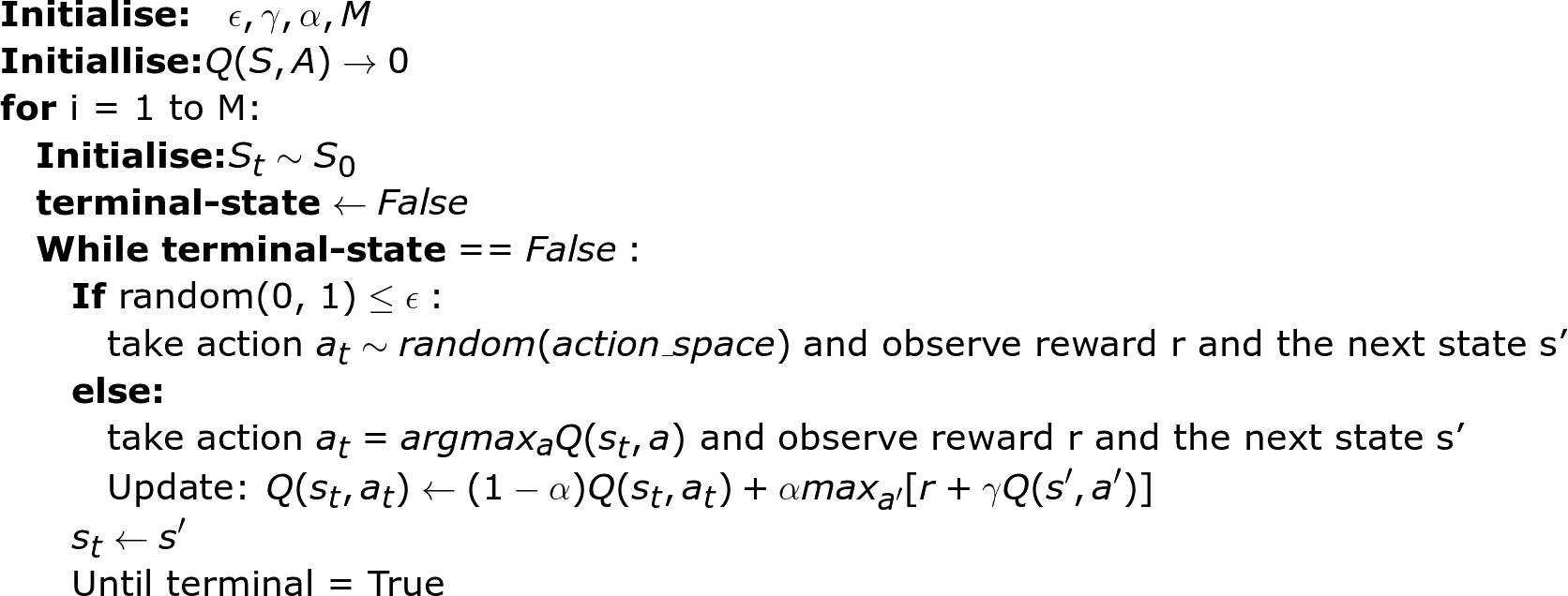
Here is the pseudo code for the Q-Learning Algorithm that you will implement:
Here are the tasks for the Q-learning:
- First complete the Q-learning block of code in the Jupyter-Notebook.
- Try varying the maximum number of episodes M from (10^3, 10^4, 10^5, 10^6, 10^7) to learn the Q-table. Observe the results of the learned Q-function using the test function which has been provided in the Jupyter Notebook. Specifically, plot the penalties incurred and the cumulative reward function as a function of iterations.
- Try varying the exploration noise, \(\epsilon\) from (0.05,0.1,0.2) and observe the changes. Plot the penalties incurred and the cumulative reward function as you varied \(\epsilon\).
Function Approximations in Reinforcement learning
You will observe that training a simple environment with state, action pairs of 500×6 elements takes a long time to converge using Q-learning. Additionally, you have to create 500×6 element size Q-table to store all the Q-values. This process of making such a large Q-table is memory intensive. You also may have noticed that this method of using a Q-table only works when the state and action spaces is discrete. These practical issues with Q-learning was what originally prevented it being from used in many real-world scenarios.
If the state space/action spaces are large, an alternative idea is to approximate the Q-table with a function. Suppose you have a state space of around \(10^6\) states and action space is continuous value from [0,1]. Instead of trying to represent the Q table explicitly, we can approximate the table with a function. While function approximation is almost as old as theory of RL itself, it recently regained popularity due to a seminal paper on a Neural Network based Q-learning algorithm called the DQN algorithm, which was proposed in 2015.
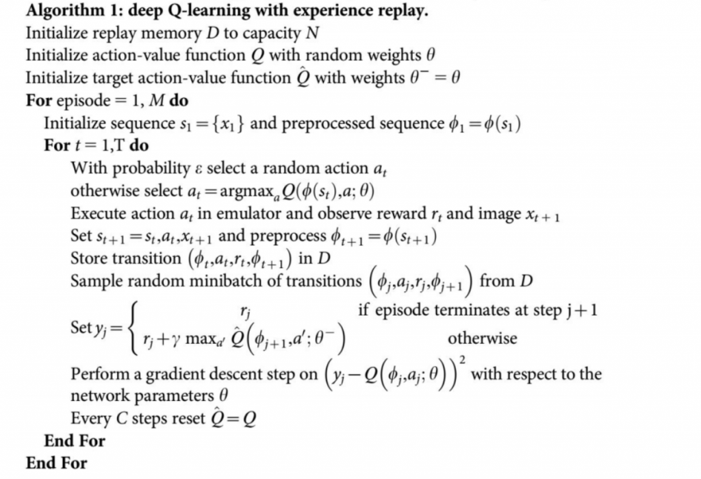
In this MP, you have been asked to implement the Deep Q-learning algorithm (DQN). The idea of this algorithm is to learn a sufficiently close approximation to the optimal Q-function using a Neural Network architecture.
We will implement the DQN algorithm as described here:
For the this part of the MP, you must provide the following tasks:
- Complete the Deep-Q learning algorithm described above in the Jupyter Notebook.
- Notice the number of Neural Net parameters in the problem. Compare this with the number of parameters in Q-learning. Based on these two things, answer the following question: Is DQN better than Q-learning for the purposes of Taxi Environment? Why or why not?
- Check the number of iterations it takes the network to converge on an “optimal” policy. Compare this with the number of iterations it took in the original Q-learning algorithm. Do you notice any difference in the executions or roll outs of these two policy approaches?
Deliverables:
You have been provided with a number of questions you need to answer after implementing each algorithm (Q-learning and DQN) respectively. You must write a report which answers the following questions
- Notice the number of Neural Net parameters in the problem. Compare this with the number of parameters in Q-learning. Based on these two things, answer the following question: Is DQN better than Q-learning for the purposes of Taxi Environment? Why or why not? If not, when will the DQN algorithm be a better solution to a RL problem
- Check the number of iterations it takes the network to converge on an “optimal” policy. Compare this with the number of iterations it took in the original Q-learning algorithm. Do you notice any difference in the executions or roll outs of these two policy approaches?
- Try varying the maximum number of episodes M from (10^3, 10^4, 10^5, 10^6, 10^7) to learn the Q-table. Observe the results of the learned Q-function using the test function which has been provided in the Jupyter Notebook. Specifically, plot the penalties incurred and the cumulative reward function as a function of iterations.
- Try varying the exploration noise, \(\epsilon\) from (0.05,0.1,0.2) and observe the changes. Plot the penalties incurred and the cumulative reward function as you varied \(\epsilon\).
Grading Evaluation
- Q-learning implementation (40%)
- Deep-Q learning implementation (40%)
- Completing the project report with question responses (20%)