Now we are going to explore the results of running Singular Spectrum Analysis (SSA) on the time series.
SSA is used to extract cycles from a time series. Specifically we are going to try and extract the (yearly) seasonal cycle.
I am going to use the Rssa package. So if you don’t have it installed.
install.packages('Rssa')
I don’t want to go over too much detail about SSA because that would take a lot of time and might not be as helpful as just going over how to use it.

So there are two steps to running SSA on R, with the Rssa package.
1. Decompose the Time Series
Then put it back together using the eigenvalues of your choice.
2. Put it Back Together
This is not scientific or mathematical vernacular for the process but my general overview.

require(Rssa)
decomposed=ssa(clean_data$avgTemp)
plot(decomposed)

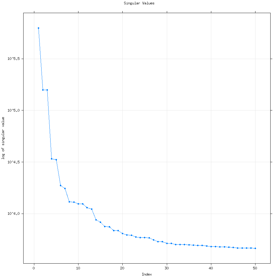
By default Rssa will use the minimum of three variables to determine the number of eigenvalues to calculate: (Length of the time series, number of time series for mSSA or multivariate SSA or 50). Every time I have used R it has wound up computing 50 eigenvalues but it can compute more if the user specifies how many.
require(Rssa)
decomposed=ssa(clean_data$avgTemp,neig=100)
plot(decomposed)

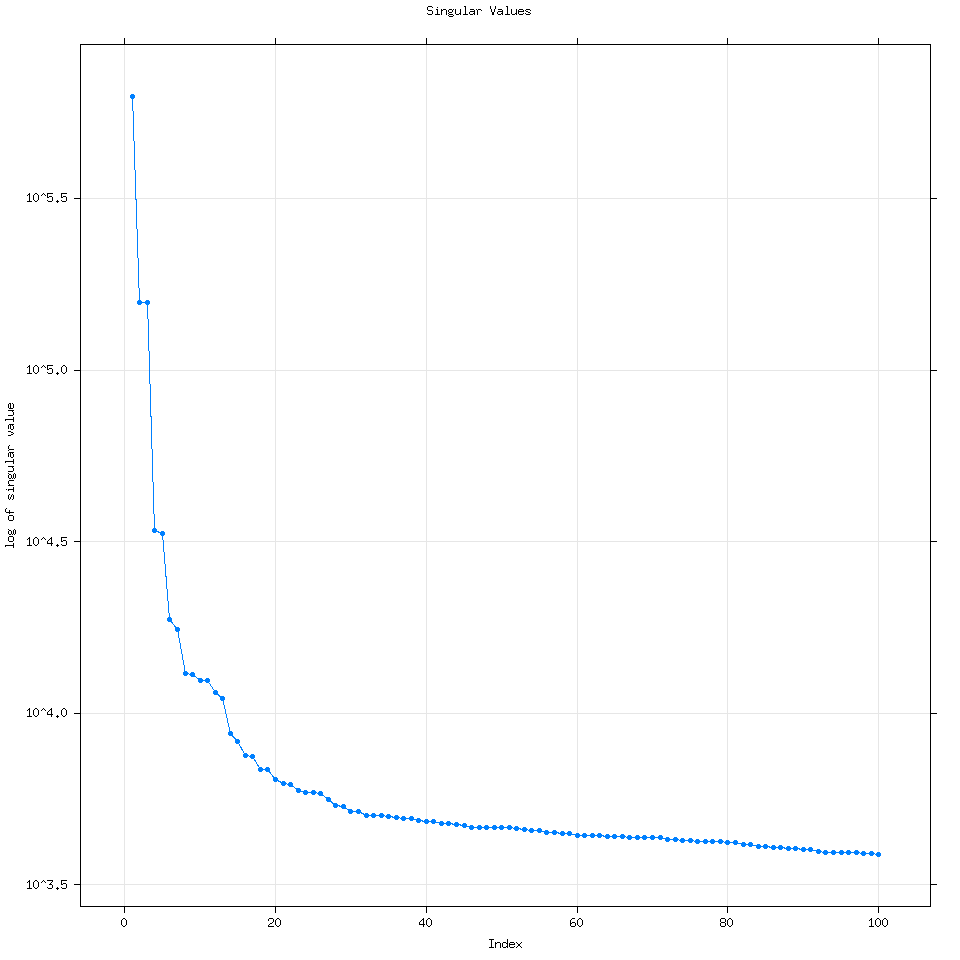
We can see that increasing the number of eigenvalues used doesn’t really change the analysis.
Going back to the vanilla 50 eigenvalue plot, how I think about this plot is that each dot corresponds to a time series. For example let’s consider the first 7 eigenvalues.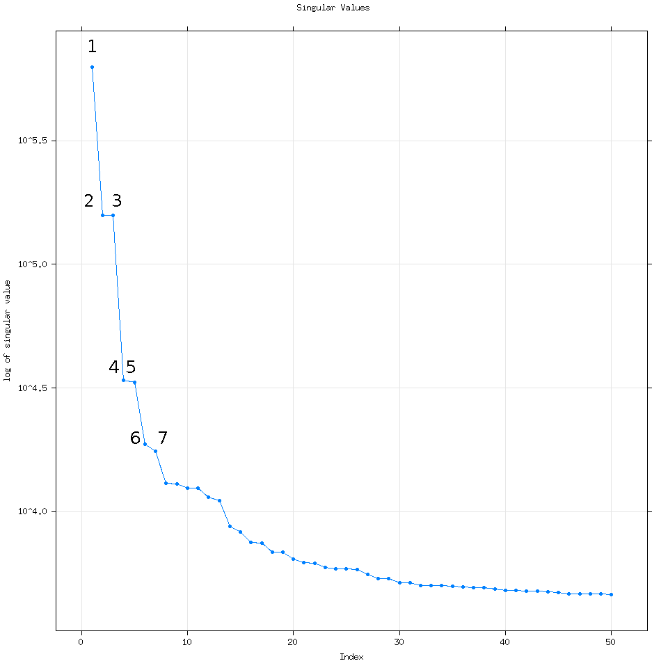
If we reconstruct the time series (putting it back together) using these seven eigenvalues let’s examine what their corresponding time series are:
SSAconstruct=reconstruct(decomposed,groups=list(one=1,two=2,three=3,four=4 ,five=5,six=6,seven=7,eight=8))
plot(SSAconstruct, plot.method = "xyplot", add.residuals = FALSE,superpose = TRUE, auto.key = list(columns = 2))

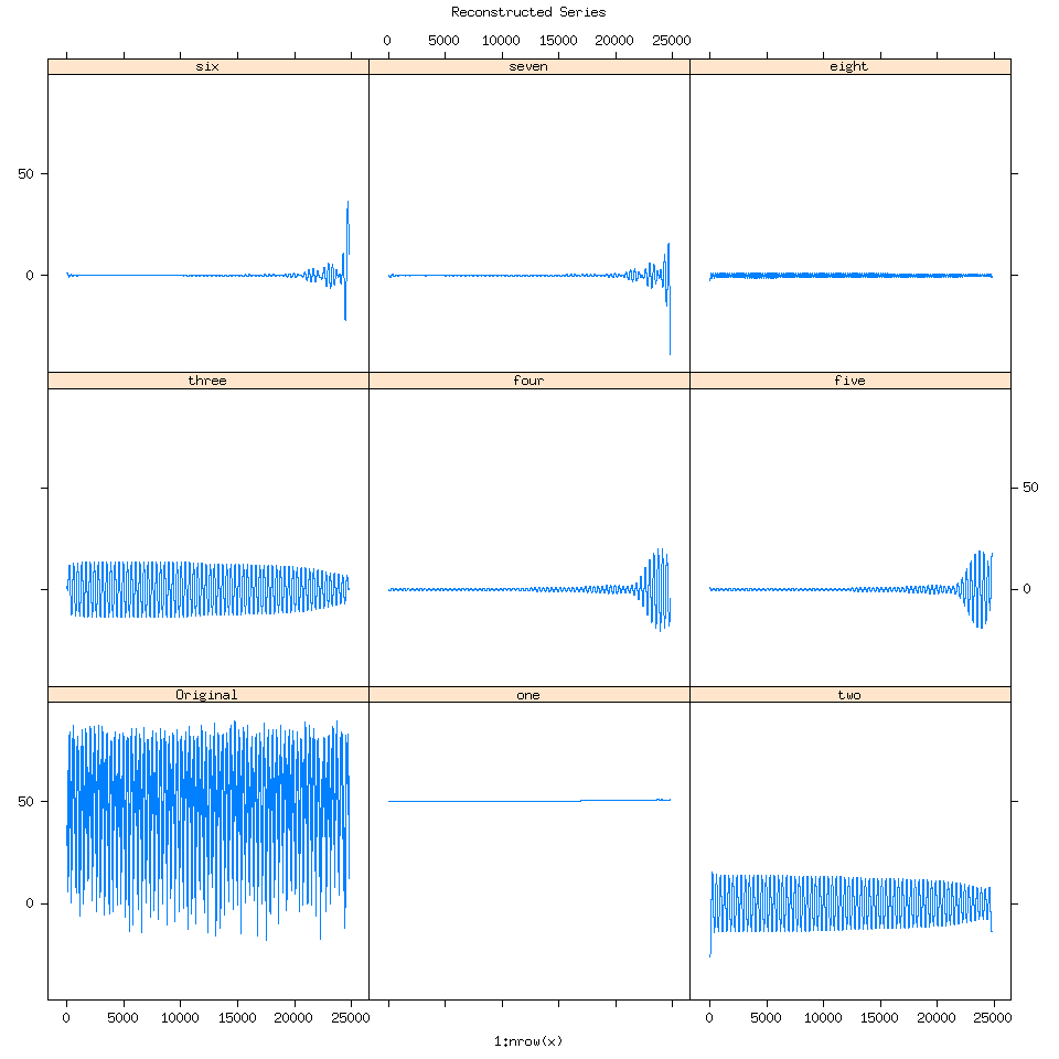
When I first saw this my reaction was “Oh wow SSA is detecting the splining we performed towards the end of the time series”.

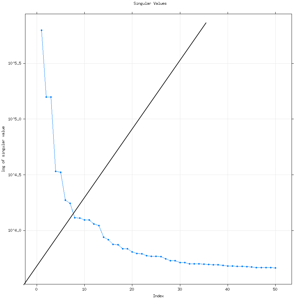
Going back to the plot(decomposed) graph, quickly, eigenvalue pairs or pairs of dots with the same magnitude are very good because they mean SSA detected the same signal but at different frequencies.
Here I have groups of dots circled to help show you what I mean. As we get to larger groups of eigenvalues with lower magnitude though it is very likely that those eigenvalues represent signals detected from noise.

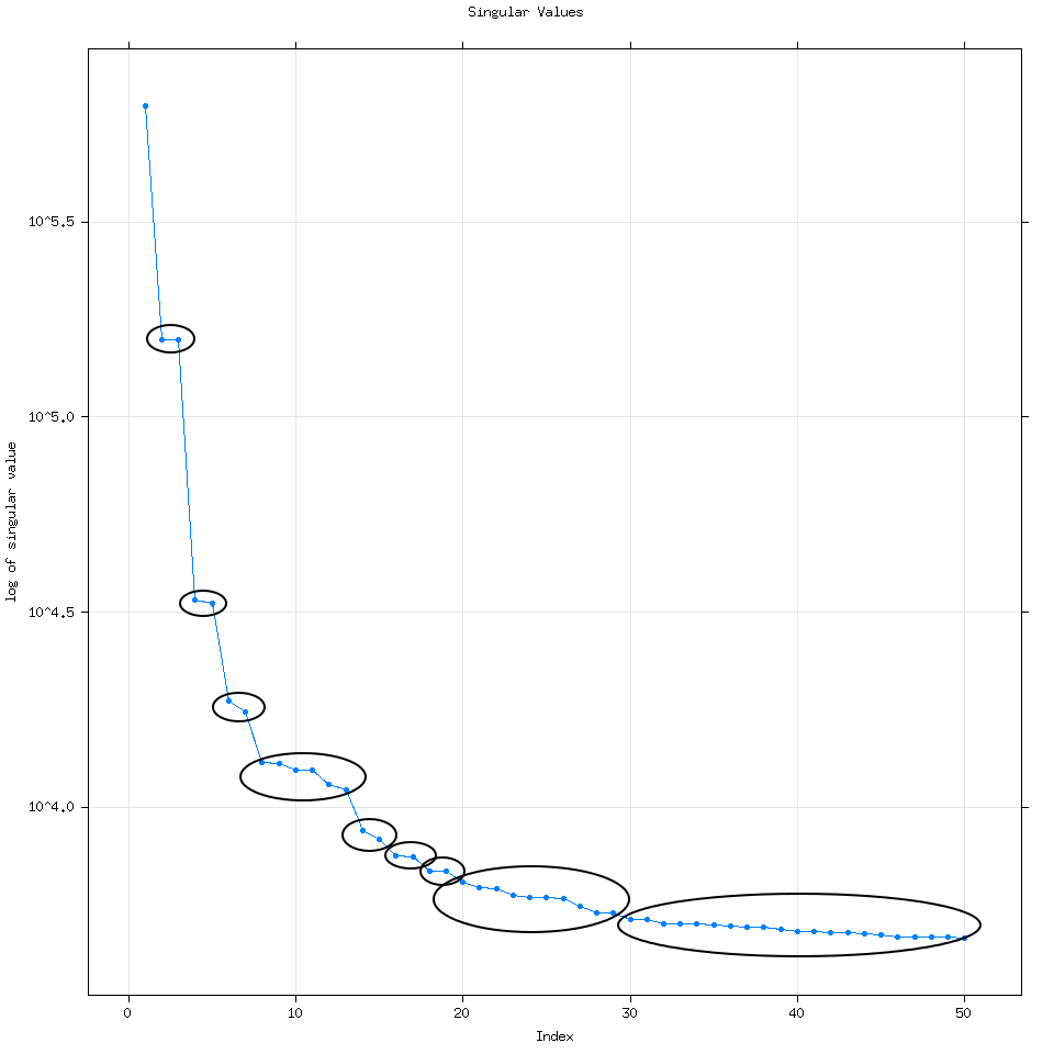
We can model the noise using SSA if we wanted to use SSA forecasting by increasing the number of eigenvalues we use to say 300 or 500.

An analogy I came up with was from economics, in the classes I had for my accounting degree, we studied consumer choice curves.
Consumer Choice Curves
Consumers try to maximize their utility or happiness.
And in this case we are trying to find the optimal balance between true signal and signals from noise, where we have just enough information to reconstruct the seasonal cycle.

One indeed has to be careful about SSA detecting signals from noise. But I’m not going to go into more significant tests here, what I will show is how do we find the eigenvalues that best represent the seasonal cycle from the data?

SSA decomposition also works on XTS variables which is great for us. But be careful Rssa chokes if you try using XTS data to create the graph of the time series for eigenvalues 1 through 7. ie this line plot(SSAconstruct, plot.method = "xyplot", add.residuals = FALSE,superpose = TRUE, auto.key = list(columns = 2))
If we try and reconstruct the time series using only eigenvalues 1-3.
decomposedXTS=ssa(avgTempXTS)
SSAconstruct1_3=reconstruct(decomposedXTS,groups=list(one=1:3))
plot(avgTempXTS)
lines(SSAconstruct1_3$one,lty=2,col='red')


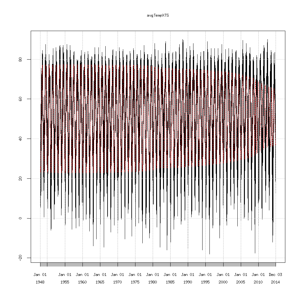
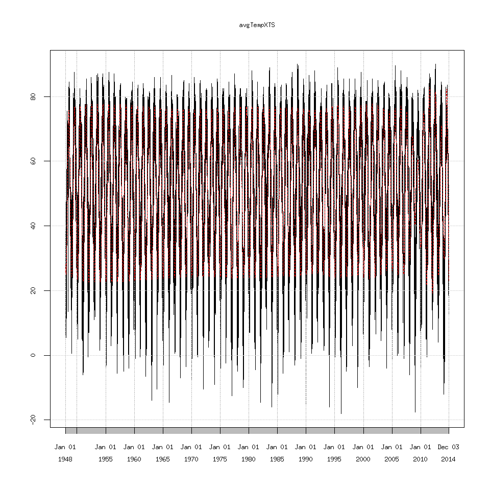
Which we can see the decreasing amplitude doesn’t match the seasonal cycle at all. I’m not going to show every graph possible because there are too many. Suffice to say eigenvalues 1 through 7 seem to recreate the seasonal cycle as best as possible but I have no idea why 2009 causes SSA to choke.
SSAconstruct1_7=reconstruct(decomposedXTS,groups=list(one=1:7))
### this is the original data plotted against the extracted signal
plot(avgTempXTS)
lines(SSAconstruct1_7$one,lty=2,col='red')

plot(avgTempXTS['2003/2013'])
lines(SSAconstruct1_7$one['2003/2013'],lty=2,col='red')

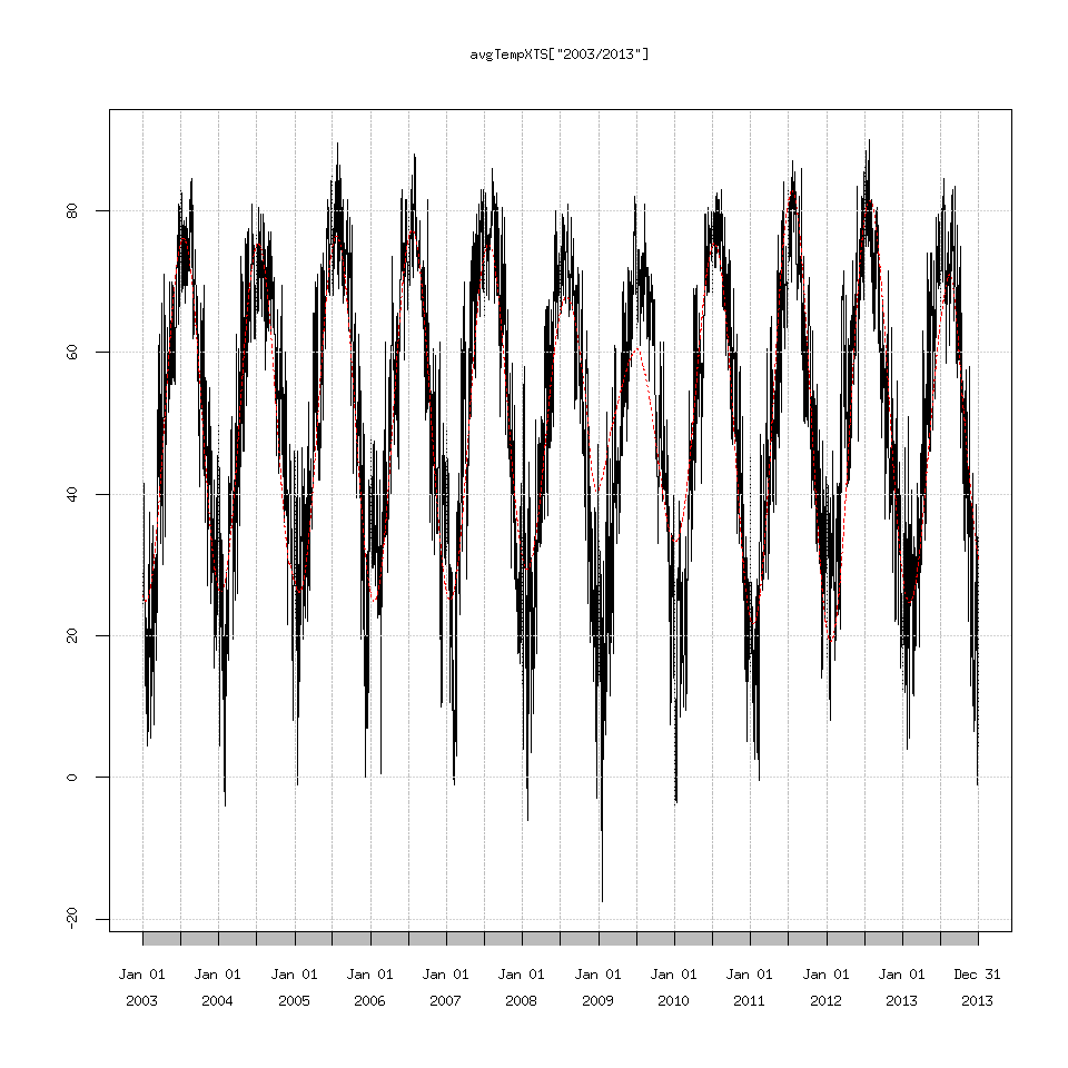
Reading the documentation for Rssa suggests that perhaps the time series is too long and I should write my own custom decomposition function.
Another option is that the trend (eigenvalue one) that Rssa detects is linear (a 50.0 to 51.0 deg F line) and SSA can struggle with extracting a linear trend.
SSAconstruct1=reconstruct(decomposedXTS,groups=list(one=1))
plot(SSAconstruct1$one)

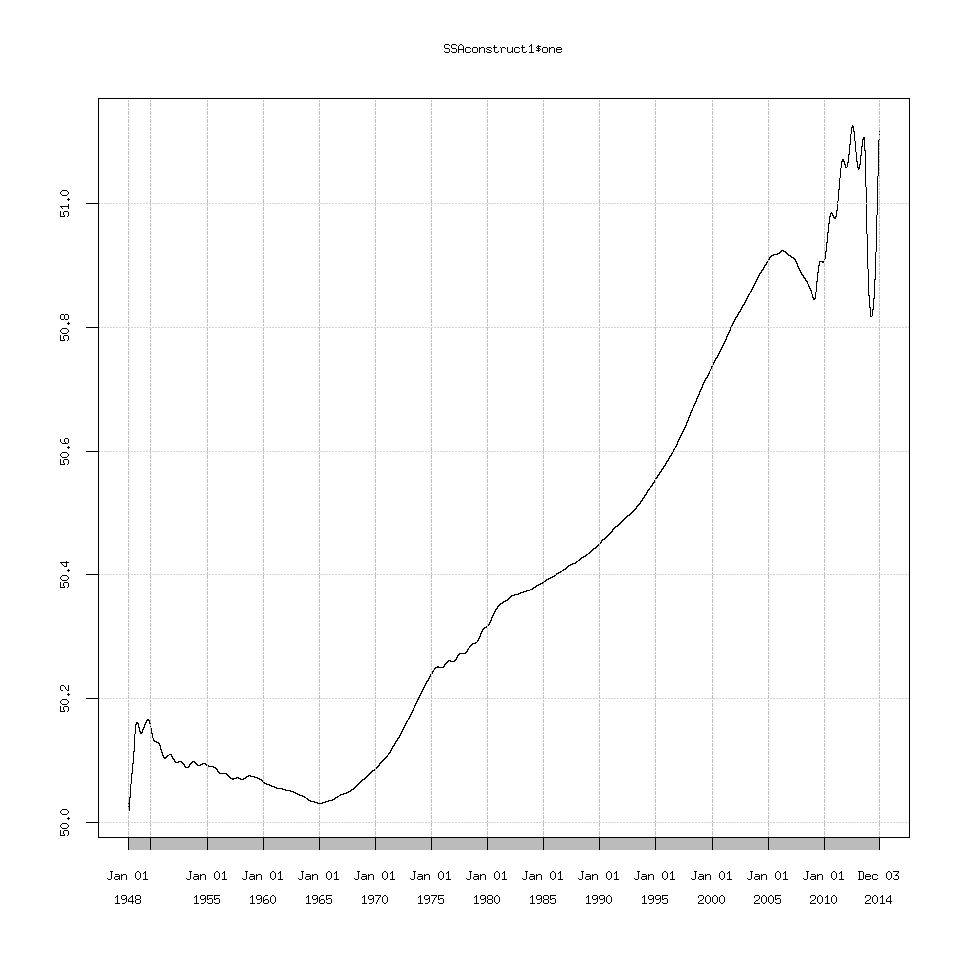
I explored changing the projection options which the documentation suggests can help extract a linear trend but I didn’t find any important changes.
The options are:
column.projector=’centering’ -> 1D SSA with centering
column.projector=’centering’ and row.projector=’centering’ -> 1D SSA with double centering
other options are: ’none’, ’constant’ (or ’centering’), ’linear’, ’quadratic’ or ’qubic’
The default is ’none’

decomposed_projected=ssa(clean_data$avgTemp,column.projector='centering')
#or
decomposed_projected=ssa(clean_data$avgTemp,column.projector='centering',row.projector='centering')


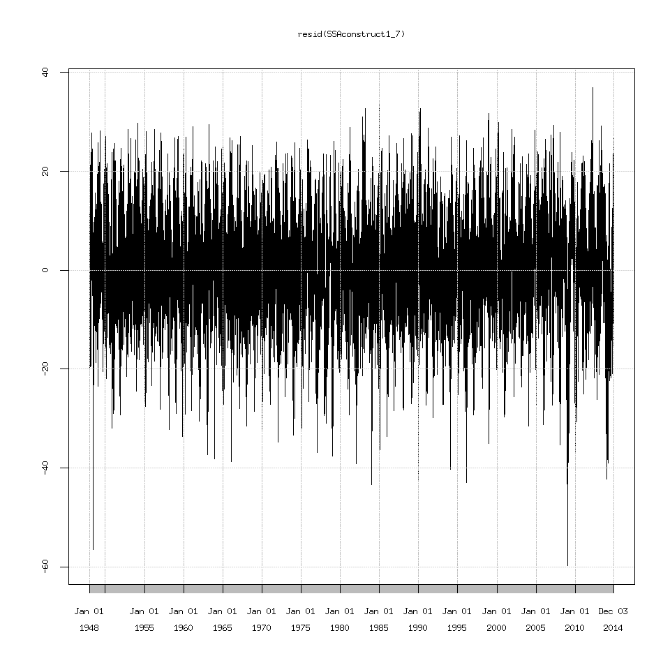
Lastly I should mention if you want to explore everything after the seasonal cycle then use the function resid() to extract them.
plot(SSAconstruct1_7$one)

plot(resid(SSAconstruct1_7))

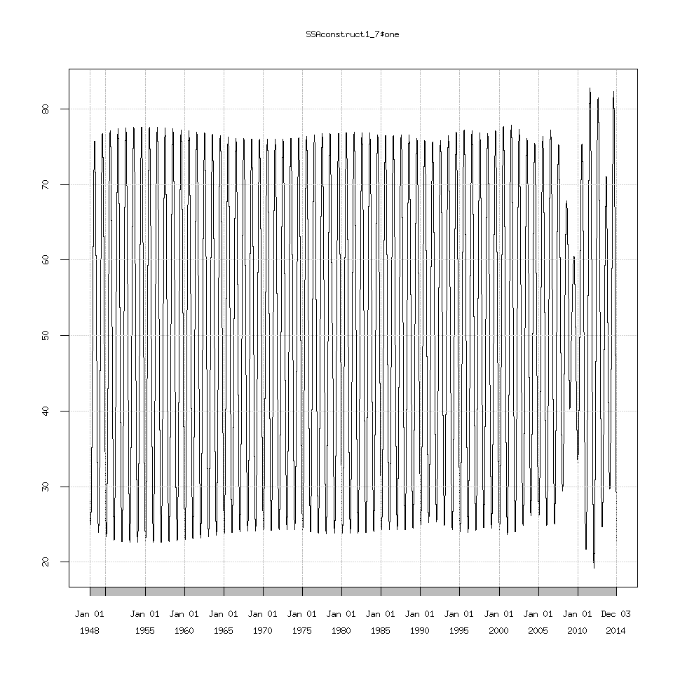
If you try plotting the signal+residuals and then overlay the signal on this graph. You will get the same graph from above where I plotted the original data and overlaid the SSA extracted signal. In other words:
#This
plot(avgTempXTS)
lines(SSAconstruct1_7$one,lty=2,col='red')
# matches this
plot(SSAconstruct1_7$one+resid(SSAconstruct1_7))
lines(SSAconstruct1_7$one,lty=2,col='red')


Anyway that is everything I have for an introduction on how to perform SSA in R, with all of the caveats or gotchas I know of mentioned.
Good luck!