
So I decided to try and spline the missing temperature data after going over na.omit(), na.approx() and na.spline() in part 1.
2. Dealing with Missing Data in R: Omit, Approx, or Spline Part 1
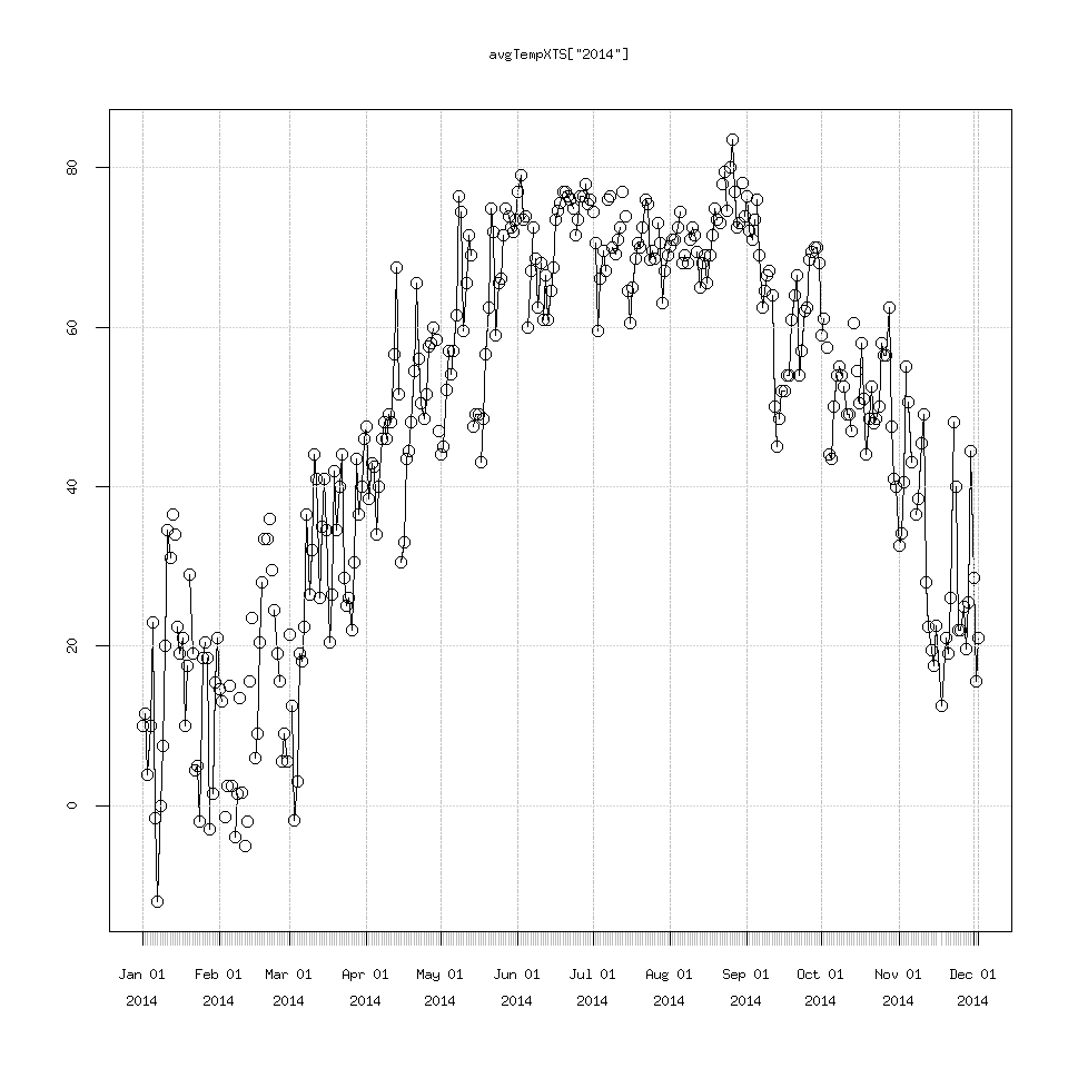
Reaching way back to step 1. Let’s revisit the missing data in February 2014 and 2013.
plot(avgTempXTS['2014'])

points(avgTempXTS['2014'])

## yup there is the missing data
## let's create a new splined XTS variable to see how polynomial interpolation does

avgTempSplineXTS=na.spline(avgTempXTS)

## to have 2 graph windows open at the same time

dev.new()

plot(avgTempSplineXTS['2014'])

points(avgTempSplineXTS['2014'])

### this looks good I don't see any crazy jumps to -200 or -300 or something

plot(avgTempSplineXTS)

points(avgTempSplineXTS)

## to compare to the original data, first change back to graph window 2

dev.set(2)

plot(avgTempXTS)

points(avgTempXTS)
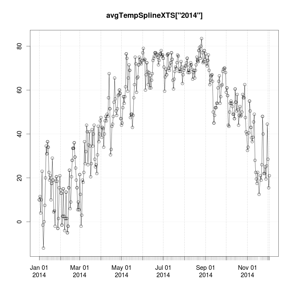
I don’t see the splined data changing any of the record highs or lows for daily average temperature so in that aspect it looks good to me.
There are more rigorous ways to check exactly what we are introducing into the data for sure, but for my purposes here (with 2% of the data missing)
this is an acceptable approach to me. The main thing to look for would be the spline output saying it was 90 degrees in January for example. Let’s quickly check for this.
### save the locations (or indices)

### where the missing data is in the vector

missingTempDataIndices=which(is.na(clean_data$avgTemp))

### output only the interpolated times

avgTempSplineXTS[missingTempDataIndices]

### scrolling quickly through this list

### the 1.23 deg in Dec 31st 1998 caught my eye

### so using the magic of XTS

avgTempSplineXTS['1998-12-25/1999-01-05']

             [,1]

1998-12-26  23.000000

1998-12-27  34.500000

1998-12-28  28.000000

1998-12-29  20.000000

1998-12-30   4.000000

1998-12-31   1.230667

1999-01-01   9.500000

1999-01-02  16.500000

1999-01-03   8.000000

1999-01-04 -10.000000

1999-01-05   0.000000

## Note for the above slice of data only

## Dec 31st 1998 is missing everything else should be good.
Apparently we have no data from Nov 2nd 2008 to May 21st 2009, that is a lot of missing data. Looking at the temperatures closely the -17.5 deg F that was interpolated for 2009-01-16 caught my eye, and the 1.23 deg F on Dec 31st 1998. Would I expect these to be accurate? No I wouldn’t expect them to be. Given the large block of missing data, perhaps using the climate average of each and every day would be better justified than relying on polynomial interpolation for such a large chuck of data.
But for the scope of this project and the missing data being only 2% of the total record, I’m going to keep it simple and use na.spline.
Let’s quickly compare it to linear interpolation and see if it does better.
avgTempLinearInterpXTS=na.approx(avgTempXTS)

avgTempLinearInterpXTS[missingTempDataIndices]

### this outputs the same temperature for 2009-01-16 = -17.5

avgTempLinearInterpXTS['1998-12-25/1999-01-05']

### But for Dec 31st 1998 this outputs 6.5 instead of 1.23 which does seem better, so it's a bit of wash

             [,1]

1998-12-26  23.00

1998-12-27  34.50

1998-12-28  28.00

1998-12-29  20.00

1998-12-30   4.00

1998-12-31   6.75

1999-01-01   9.50

1999-01-02  16.50

1999-01-03   8.00

1999-01-04 -10.00

1999-01-05   0.00
Rather than declaring one method superior to the other, let’s take another perspective: dealing with missing data has already introduced some uncertainty into the analysis and we haven’t really done anything yet. I view this as another parameter to consider. Either na.omit(), na.approx() or na.spline() depending on how uncomfortable you are with interpolating data. If you want to be absolutely sure it doesn’t change the output of what you’re looking at, where possible, you would want to re-run your test or plot with all three of the NA functions and see if the results differ. If the results don’t change under all three cases then I would argue that the results are robust.
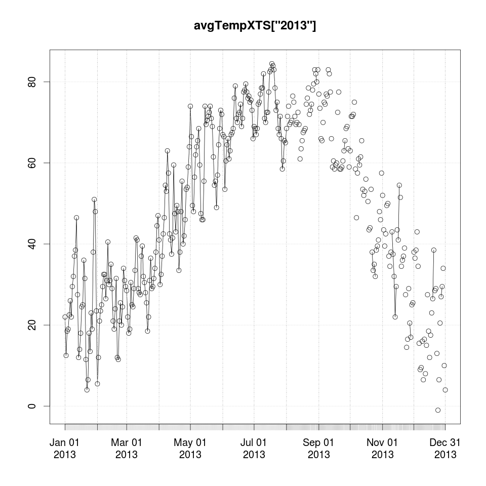
Next let’s compare 2013 as well.
dev.set(2)

plot(avgTempXTS['2013'])

points(avgTempXTS['2013'])
dev.set(3) # or dev.new() if it doesn't exist

plot(avgTempSplineXTS['2013'])

points(avgTempSplineXTS['2013'])
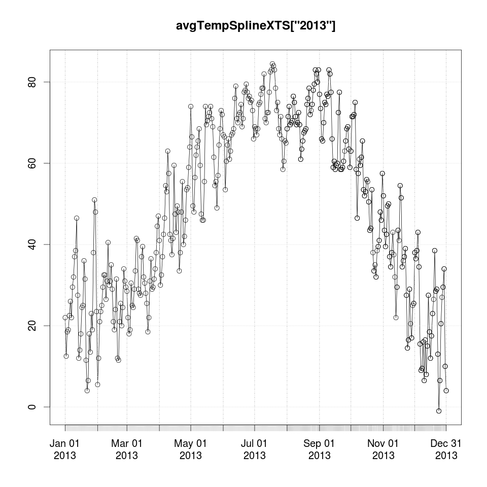
The results for the second half of 2013 look really good.
Lastly about the missing data for precipitation, I would argue the best step if we don’t want to throw out 25 days of temperature data because of missing precip data is to just set the missing precip data = 0. Interpolating either linearly or splining a daily sum precipitation time series is wildly inappropriate. Unless we had radar data to suggest it was raining continuously over Galesburg before, during and after the missing days.
To update the dataframe appropriately.
### before

summary(clean_data)

###

clean_data$PRCP[is.na(clean_data$PRCP)]=0

clean_data$TMAX=na.spline(clean_data$TMAX)

clean_data$TMIN=na.spline(clean_data$TMIN)

clean_data$avgTemp=na.spline(clean_data$avgTemp)

### after

summary(clean_data)
Now we have to remember we splined the data. But at long last we are ready to rumble!
Stay tuned!
See the code recap for what we have so far.
2b Complete Code Recap