Problem 1

Part 1

For differential equations without analytical solutions, we can use numerical approximation in order to estimate the solution. One simple method is called Euler’s method. In this section, we will use Euler’s method on a differential equation that does have an analytical solution to show the numerical error that is intrinsic to this method. The model we will be analyzing is the Mathusian/Verhulst logistic population model, which written as:

\[\frac{{dN}}{{dt}} = \alpha N\left( {1 – \frac{N}{K}} \right)\]

where, N is the population, t is time, α is rate constant with dimensions of inverse time, and K is the carrying capacity. Now, we can approximate this differential equation using a finite element, so

\[\frac{{\Delta N}}{{\Delta t}} = \alpha N\left( {1 – \frac{N}{K}} \right)\]

This finite element solution approaches the differential equation when the time step is infinitesimally small. We can rewrite this equation using the forward difference scheme with index, i.

\[\frac{{\left( {{N_{i + 1}} – {N_i}} \right)}}{{\left( {{t_{i + 1}} – {t_i}} \right)}} = \alpha {N_i}\left( {1 – \frac{{{N_i}}}{K}} \right)\]

This solution is explicit for N_i+1. Given that we know the value at index, i, we can specify a time at index, i+1, and solve the equation for N_i+1.

\[\left( 1 \right):{N_{i + 1}} = {N_i} + \left( {{t_{i + 1}} – {t_i}} \right)\alpha {N_i}\left( {1 – \frac{{{N_i}}}{K}} \right)\]

This equation (1) can be used to solve for all N during time period, t, as long as we are given an initial condition. We can compare this to an analytical solution, which is given below, equation (2).

\[\left( 2 \right):N = \frac{{K{N_o}{e^{\alpha t}}}}{{K + {N_o}\left( {{e^{\alpha t}} – 1} \right)}}\]

Part 2

To implement equation (1) in to a numerical code, we need to utilize for-loops. A for-loop, loops through a piece of code a specified number of times. Additionally, a counter/index can be used within the for loop. For our explicit numerical equation, (1), we can write the code in a loop with index, i, and for a total number of loops, M. The code looks like

import numpy as np #import library

n = 365 #number of times the code loops
dt = 1.0 #timestep
alpha=0.1#growth rate
K=2000.#carrying capacity
model = np.zeros((n,2)) #model, dependent
#and independent variables

model[0,0]=1#dependent initial condition
model[0,1]=100.#independent initial condition

for i in xrange(1,n):
     model[i,0]=model[i,0]+dt
     model[i,1]=model[i-1,1]\
     +dt*alpha*model[i-1,1]*(1-model[i-1,1]/K)

Part 3

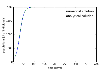
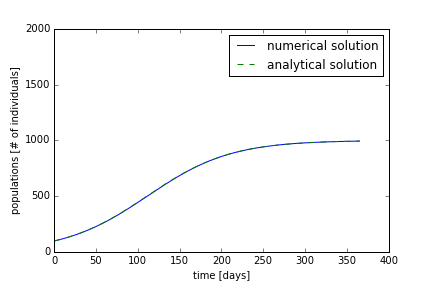
Using the code from part 2, we can simulate the growth of a certain species. We will use a carrying capacity of 2000 individuals and an initial population of 100 individuals. On the first day, we want to have a growth of individuals of ten people.  This means that (100 * α = 10); therefore, alpha is 0.1. We will iterate the growth for 365 days. With these parameters, the numerical and analytical solution are shown in Figure 1. The population starts at the carrying capacity and reaches the equilibrium carrying capacity near 100 days. The analytical solution and numerical solution differ slightly, but are in quite good agreement.

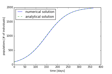
By adjusting the parameters, we can change how the species grows. If we reduce the value of α, the growth rate, we will have a population that grows slower, shown in Figure 2. We see that it takes the population almost a year to reach the carrying capacity.

In one more test, we will use the same growth rate as in Figure 2. Instead of using a carrying capacity of 2000, we will use a carrying capacity of 1000, half of the first one. This is shown in Figure 3. Here the initial growth of the population is similar to the growth in Figure 2; however, it reaches a smaller final population. With Figure 2 & 3, we see the effects of the parameters K and α in the model.

Problem 2

Part 1

Using a similar modeling frame work as in problem 1, we can create a box model to represent the number of Coho salmon in Lake Michigan. First, we need to get initial conditions and some rates for our model. We know that approximately 5.6 million Coho and Chinook are stocked in Lake Michigan each year. About 3/4 of the fish are Coho, therefore 4.2 millions Coho fish are stocked each year. Assuming no fish are killed and no fish are birthed, the maximum number of fish that can be in the lake at 3 years is 12.6 million fish. We will use this as our initial condition because it is a ball park value for the amount of fish in the lake. The average daily rate is the the annual stocking rate divided by 365.25 days. The daily stocking rate is 11499.0 fish per day.

Part 2

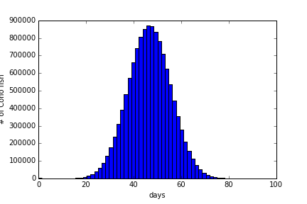
The Coho fish migrate into tributaries from the lake; we will assume that about 1/3 of the fish migrate to the tributaries over a 60 days during the months of October and November. Around Halloween, the maximum amount of fish will migrate from the lake to the tributaries. We will assume the distribution of the fish will migrate according to a normal distribution. The follow code was provided to generate a plot and text file of the migration rates over the 60 days. Here is the code.

#import libraries
%matplotlib inline
import numpy as np
from matplotlib import pyplot as plt
import random

#initial population
N0 = 12600000.0
#set up numpy array
x=np.zeros(int(N0))
#standard deviation
sigma = 9
#choose normal random numbers with mean 0.0
# and standard deviation 1.0
for i in xrange(0,int(N0)):
    x[i] = random.gauss(0.0,1.0)# Defining the standard deviation 
#multiple the numbers by the standard deviation
Na = sigma*x 
#find minimum value and subtract all values by it. min will be zero
Nb = np.amin(Na) 
Nc = Na - Nb  
#create histogram, and make 60 bins
Nd, bins, patches = plt.hist(Nc,60)
#divide migration rates by 3 because 1.3 of pop migrates
N_mig = Nd/3 
#make array for days
X = np.zeros((60,1))
for i in range(60):
    X[i] = i + 1
#save files as txt file
np.savetxt('fish_migration.txt'\
,np.transpose([X[:,0],N_mig]), fmt='%8d' )

This code produces the following histogram, Figure 4.

Part 3

In this part, we will apply a death rate to the fish in the lake. The equation is as follows

\[{\omega _N} = {\omega _{\min }} + {\omega _1}N\]

where ω_N is the death rate in units of days^-1 that makes up the first order death rate, ω_min is the minimum death rate in the absence of fish, and ω₁ is a rate constant that depends incorporates the dependence of the population in units of (days*fish)^-1 that makes up a second order death rate. In thinking about the rate constants, we must understand what we expect the population to do from day 1. Since our initial condition is the maximum population the fish can be, we can assume that that population will most likely decrease. Without fish migration, the conservation equation at equilibrium, dN/dT = 0, is

\[\frac{{dN}}{{dt}} = 0 = {r_{daily}} – N{\omega _N}\]

where r_daily is the daily stocking rate. The substitution of our formulation for the death rate results in a quadratic equation.

\[{N^2} + \frac{{{\omega _{\min }}}}{{{\omega _1}}}N – {r_{daily}} = 0\]

with solution (positive root),

\[\left( 3 \right):N =  – \frac{{{\omega _{\min }}}}{{2{\omega _1}}} + \sqrt {{{\left( {\frac{{{\omega _{\min }}}}{{2{\omega _1}}}} \right)}^2} + \frac{{{r_{daily}}}}{{{\omega _1}}}} \]

We should note that the preceding analysis ignored the migration rates. Migration rates remove 1/3 of the initial population, a significant portion of fish population. As we see in the equation, increasing either ω parameters will decrease the final equilibrium population, i.e. the carrying capacity.

Now, let us ignore the migration rate and the ω₁ constant. Let us say that the initial condition is the maximum population that the lake can sustain. This means at this population, dN/dT = 0. This means ω_min = (11499.0 fish/day) / 12.6 millions fish = 0.0009126 days^-1. Now if we want a stable fish population, we can solve equation (3) for N = 12.6 million fish and 0 fish. This means that the final population without migration of fish will be in between the initial condition and zero. From our analysis, we see that the limits for ω₁ are from zero to infinite. At very small values of ω₁, the equilibrium population is 12.6 million fish and when ω₁ is infinite, the equilibrium population is 0. In between these values shows the following plot (Figure 5):

We see that in between ~ω₁ = 1.0 x 10^-8 and 1.0 gives reasonable stable values of fish. This means that ω_min controls the upper limit of the population and ω₁ sets what the value will be in between the upper limit and zero.

Part 4

Now, with all the parts of the problem, we can fully model the fish with stocking, migration, and death using the following conservation equation:

\[\left( 4 \right):\frac{{dN}}{{dt}} = {r_{daily}} – {r_{migration}}\left( t \right) – {\omega _{\min }}N – {\omega _1}{N^2}\]

where r_migration is the migration rate, which is a function of time. This conservation equation (4) can be discretized and written in a explicit form similar to equation (1). This is equation (5);

\[\left( 5 \right):N\left( {{t_{i + 1}}} \right) = N\left( {{t_i}} \right) + \Delta t\left[ {{r_{daily}} – {r_{migration}}\left( {{t_i}} \right) – {\omega _{\min }}N\left( {{t_i}} \right) – {\omega _1}{N^2}\left( {{t_i}} \right)} \right]\]

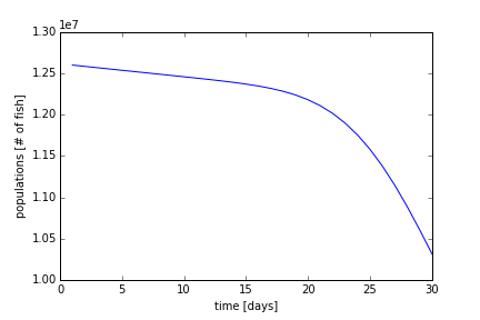
The numerical code is listed in the supplementary materials. Using ω₁ = 1.0 x 10^-10 (days*fish)^-1, ω_min = 0.0009126 days^-1, r_daily = 11499.0 fish/day, and initial condition of 12.6 million fish, we can generate Figure 6. We see that over the 30 days, the decay of the population starts out slow and increases at the 20 day mark. This is most likely due to the migration rate of the fish increasing, near the peak of the normal curve. 20 days is about one standard deviation from the mean of 30 days.

Part 5

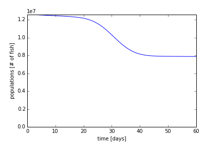
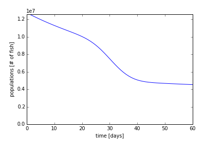
To ensure that the fish population does no drop under zero, due to the migration, we set a condition that makes the minimum population equal to zero. That is, when the population goes below zero, we set it zero. Now using a time period of 60 days, we will re-run our simulation in part 4 in Figure 7. The decay of the population is maximum at 30 days, where the migration rate is constant. The population begins to stabilize at 60 days, where it will decay to around ~7 million fish according to equation (3).

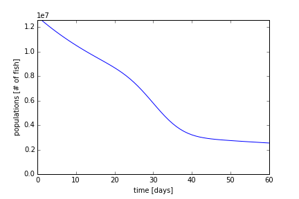
Using a ω₁ = 1.0 x 10^-9 (days*fish)^-1, one order of magnitude greater, we expect the equilibrium population to be lower (Figure 8). Here, the stable population at 60 days was near ~3 million fish. We also see that the initial rate of decay in the first 5 to 10 days was faster than in Figure 7.

Last, using ω_min = 0.009126 days^-1, one order of magnitude greater, we plot Figure 9. With a greater death rate, the decay rate (slope) increases even more. The slope, unlike in Figure 7, the is of the order of decay due to the migration of fish to the tributaries. The equilibrium population has not been reaches after 60 days, and from equation (3), it should reach about ~1 million fish.

Part 6

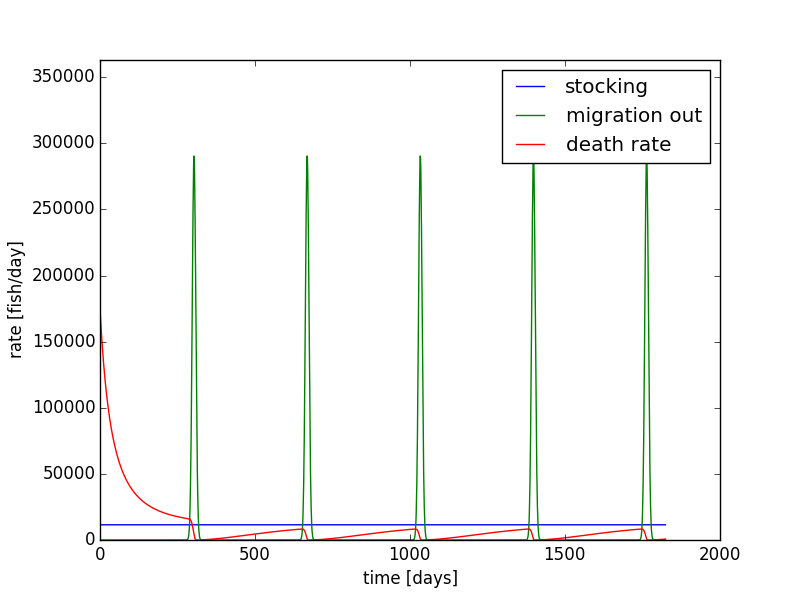
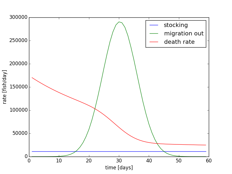
Using the same parameters from Figure 8, we can show the rates of migration, stocking, and death on each day (Figure 10). This plot shows us which term changes the population. Here we see the migration rate out has the same pattern as seen in Figure 4. The migration rate is initially very small, peaks at 30 days, and drops back to small rate at 60 days. The death rate starts out relatively large, and it decreases as time progresses. Since the death rate is a function of the population, we see a significant drop near day ~25 because of the population drop due to migration. The stocking rate is constant at 11499 fish per day. The death rate approaches the stocking rate; when they match, the population has reached a steady equilibrium.

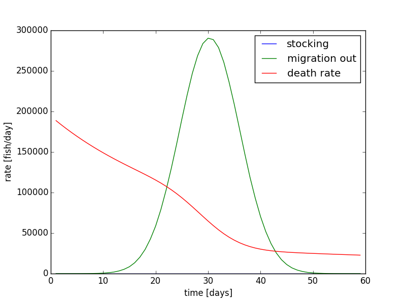
If the stocking rate is added all at the beginning of the 60 day time period, 689940 fish will be added at once. on day one. The population evolution is shown in Figure 11, and the rates are shown in Figure 12. Overall, the evolution in Figure 11 does not look very much different from Figure 8. The other differences are that the rate of decay is slightly larger in the beginning days, and the end population on day 60 is sightly lower. The initial rate is larger in Figure 11 and 12 because the population is higher. The initial condition is larger in the simulation where all the fished are stocked on a single day, and the final condition is lower. Therefore, the rate of decay of the fish is larger. Since the equation is non-linear, it matter more about how and when the fish are added instead of the total amount. These dynamics are important for building models, and how certain assumptions are made and dynamics are implemented need to be evaluated.

Extra

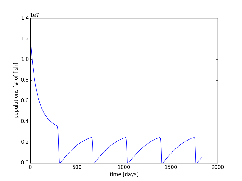
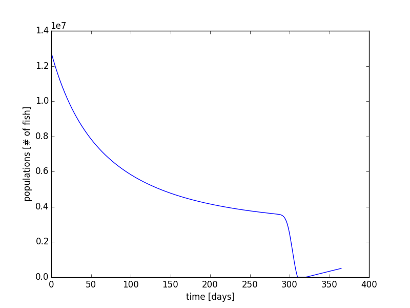
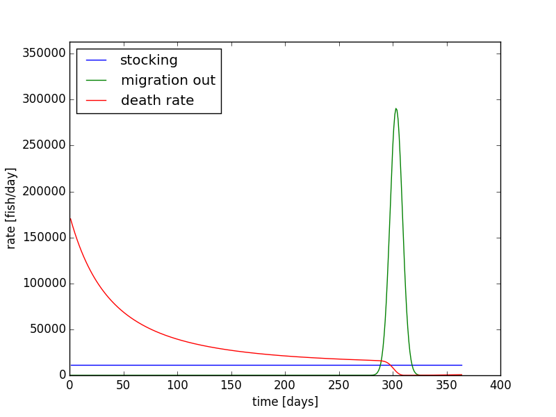
In this extra section, I have modified that code to simulate the fish population in the earlier part of the year and later part of the year. We will only have the migration rates applied during the months of October and November. In the other months, the only changes in fish population are due to the stocking and the deaths rate of the fish.  This can be completed within the code using a simple if statement. Using ω₁ = 1.0 x 10^-9 (days*fish)^-1, ω_min = 0.0009126 days^-1, r_daily = 11499.0 fish/day, and initial condition of 12.6 million fish, we can simulate the Coho fish populations over an entire year (Figure 13 & 14).

Next, we can also increase the time period to multiple years. Using our same code with the implementation of the modulus function in python, we can allow for the migration of fish every October and November in each year. Using the same parameters, we can run the simulation for 5 years (Figure 15 & Figure 16). What we see is that the population reaches a sort of equilibrium. It is not a steady state equilibrium where the population is steady and constant over time. Instead, after a few years, the population begins to follow a steady form each year with a rise in the beginning of the year, and a mass migration towards the end of the year.