Problem 1
In this exercise, we were given data that shows the growth of individual bacterium over time. In order to understand the growth dynamics in between data points (interpolation) and beyond the data points (extrapolation), we need to fit a numerical model to the data. In this problem in particular, we will fit a linear regression by linearizing the data and a non-linear regression. Both regressions that we will use are packages within the SciPy library.
Part 1
Before, fitting models, we needed to import the data into the our code. Since numpy arrays are relatively easy to work with, we will import the data, which is in a text file, as a numpy array. The following code did this:
import numpy as np

expodata = np.loadtxt('./expodata.txt',skiprows=1)

#expodata is the numpy array
#np.loadtext loads the .txt file as numpy array
#./ chooses the current working directory
#expodata.txt is the data .txt file
#skiprows=1 skips the first row, which contains the headers of the dataset
It is helpful to have labels on the columns of our data, so the modeler can read the data. Skiprows = 1 allows us to skip that header in the first row, so the numpy array only contains the data.
Part 2
In this part, we want to write an external function that we will able to use for future programs. This program, “exponential.py”, is a function that allows the user to input two parameters and an array. An exponential function is written as
\[\left( 1 \right):X\left( t \right) = X\left( {{t_o}} \right){e^{at}}\]
where X contains our data for the bacterium amount, X(to) is the initial X value at time zero, t is time, and a is the growth/decay date (in this case, growth). Our exponential function will take three arguments. The first is is the dependent variable, t. The second and third are X(to) and a, respectively. This contains the essential parameters to model the exponential function. This provides the independent variable data to create the dependent variable array, X. X is the output of the function. The function is written as:
import numpy as np

#b contains the exponential parameters
#time_array contains independent array
#thing_array contains dependent array
def exponential(time_array,Xo,a):
    thing_array = Xo*np.exp(a*time_array)
    return thing_array
Part 3
The work in part 1 allows us to import the data into a workable format. The work in part 2 allow us to specify a set of parameters and an array of the independent variable to generate an array of the dependent variable using an exponential model. We can estimate the parameters from a linear regression using the data. In python, we used the stats.linregress package in SciPy. The calling of the function is shown below
[slope,intercept,r_regres,p_regres,sterr] = stats.linregress(expo_log)
The function outputs a slope, intercept, R value, a p-value, and standard error, repectively. The only input is a two column array that holds the independent and dependent data. A linear regression is able to fit values for two parameters, m and yo, in the following equation:
\[\left( 2 \right):y\left( x \right) = mx + {y_o}\]
where y is the dependent variable and x is the independent variable. Obviously, this equation is not exponential. To fit our data, we must transform it, i.e. linearize it. By taking the natural log of both sides of equation 1, we can linearize the equation to look more like equation 2.
\[\begin{array}{c}\ln \left[ {X\left( t \right)} \right] = \ln \left[ {X\left( {{t_o}} \right){e^{at}}} \right]\\\ln \left[ {X\left( t \right)} \right] = at + \ln \left[ {X\left( {{t_o}} \right)} \right]\end{array}\]
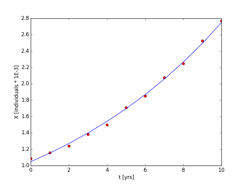
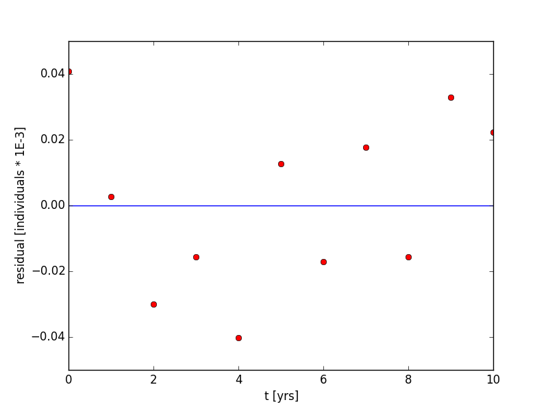
Therefore, the slope, m, is a and the intercept, yo, is ln[X(to)] when we linearly regress t vs. ln(X). Therefore, a = m and X(to) = exp( yo). The results of the linear regression is shown in Figure 1 and Figure 2. a = 0.0965 yrs-1 and X(to) = 1.047 individuals * 1e-3. The R2 value is 0.9967, which indicates a good fit. Additionally, the p-value of the regression is 1.72e-12, which indicates that there is a definite correlation. Last, the residual plot in Figure 2 shows no apparent patterns or bias; meaning, our choice in the model, an exponential model, was good. The code to generate this plot is shown in the supplementary material.
Part 4
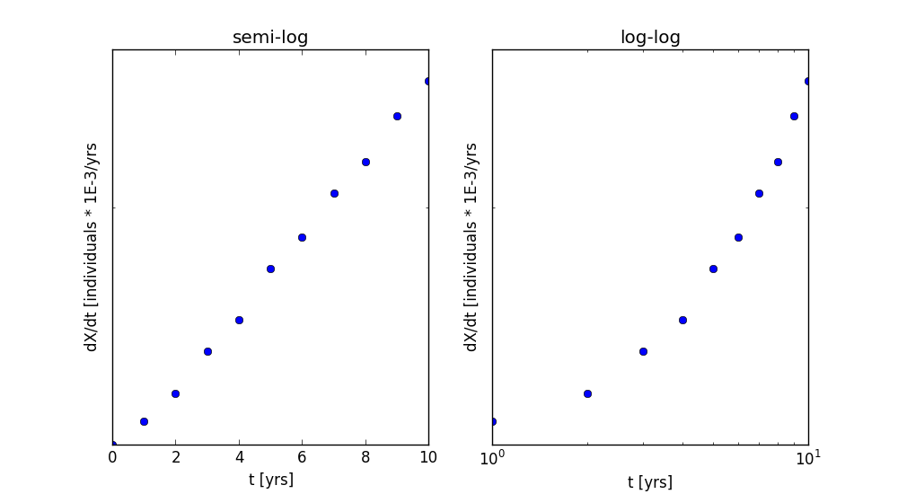
This section is similar to part 3, but instead of using a linear regression to fit the data, we will be using a non-linear regression. In a linear regression, the data must be transformed to a form that is linear. If the function is linear, exponential, or a power function, the function can be transformed using natural logs. However, for functions that are more complicated and that cannot be linearlized, this will not work. In a non-linear regression, the user specifies the function form and the parameters they want to fit. This will work for a broader array of functions. This poses a problem, though; we guess the function form before proceeding. When searching for the function, we can manipulate the axes of plot of the data to guess the function. If the data is linear in linear space, the function is a linear one, y = mx + b; if the data is linear in semi-log space, the function is an exponential one, y = y(xo)exp(at); and if the data is linear in log-log space, the function is a power function, y = axb. We already see that the data is not linear in linear space, so to guess the function we will look at the data in semi-log and log-log space (Figure 3). From these plots, we see that the data is fairly linear in semi-log space, which corresponds to an exponential function.
To specify the function form, we wrote a function within python. The function was inputted with the parameters and the independent variable, and it would output the dependent variable. This function is the exact same function, exponential.py, that we wrote in part 2. When fitting the data with a non-linear regression, the results of the fit are the parameters. Unlike the linear regression, the non-linear regression gives us the parameters, X(to) and a, directly, and we do not have to transform them. The non-linear regression was called in python using the optimize.curve_fit package in SciPy. The function was called as
b,pcov = optimize.curve_fit(exponential,expodata[:,0],expodata[:,1])
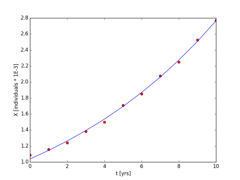
We had to input the function name, the independent variables, and the dependent variables. The code outputted the two parameters in our exponential function in the array, b, and some statistics on the variance and covariance of the parameter estimates in pcov. The resulting non-linear regression is shown in Figure 4. a = 0.0980 yrs-1and X(to) = 1.038 individuals * 1e-3. The code use to generate this plot is listed in the supplementary materials.
By manipulating the exponential equation (Equation 1), we can estimate a time that it would take for the population to double its final measured size. This time is time independent, and we will prove it below. First some definitions. tf = final time and td = doubling time.
\[\begin{array}{c}X\left( {{t_f}} \right) = X\left( {{t_o}} \right){e^{a{t_f}}}\\X\left( {{t_f+t_d}} \right) = X\left( {{t_o}} \right){e^{a\left( {{t_f} + {t_d}} \right)}}\end{array}\]
If X(tf+td) = 2X(tf) ,
\[\begin{array}{c}X\left( {{t_d}} \right) = X\left( {{t_o}} \right){e^{a\left( {{t_f} + {t_d}} \right)}} = 2X\left( {{t_f}} \right) = 2X\left( {{t_o}} \right){e^{a{t_f}}}\\{e^{a\left( {{t_f} + {t_d}} \right)}} = 2{e^{a{t_f}}}\\{e^{a{t_d}}} = 2\\{t_d} = \frac{{\ln \left( 2 \right)}}{a}\end{array}\]
Since, tf was canceled out, the doubling time is independent of time. Second, the doubling time can be estimated as the natural log of two divided by the rate constant, a. This means td = 7.07 yrs. If we take the amount at the final time, 10 yrs, and double it, we can estimate the time it takes for the population to reach double the final population by back-calculating. We can solve for this time with the following equation:
\[{t_{{\rm{2}}{{\rm{X}}_f}}} = \frac{1}{a}\ln \left[ {\frac{{2{X_f}}}{{X\left( {{t_o}} \right)}}} \right]\]
This equation results in the estimate that it will take 17.09 yrs for the population to reach double the final population at time = 10 yrs.
This is an estimate, and there may be some uncertainty attached to it. First, our model could be incorrect; meaning, the data follows a different function other than an exponential function. This would mean the estimate may not hold after the 7.07 years it takes for the population to double. Additionally, if the model is not exponential, the doubling time would be dependent on the actual time. Second, many population models contain a carrying capacity. Meaning, the maximum population that can be generated. This can occur due to environmental limitations. Here the population would initially grow at an exponential rate until it reaches the carrying capacity, where it tails off. Depending on the carrying capacity and how close it is the to final population at ten years, the estimate of the doubling time could be off. The colony therefore would not reach double the size in the predicted time.
Problem 2
Using the same two programs from part 3 and part 4, we can run similar regressions on a different data set. Instead of a data set showing exponential growth, we will analyze one with exponential decay. This data set contains the radioactive decay of Polonium-210 with units in becquerel over a period of days. In this problem, we will use both the linear and non-linear regression and compare them. Again we will use stats.linregress and optimize.curve_fit packages from SciPy. The stats.linregress function was called the same way as in part 3, but we needed to add extra information to the optimize.curve_fit function. Because the data set is decaying, the optimize.curve_fit could fail if it assumes a positive growth constant, a. The function allows for an initial guess. If we input an initial guess with our first X value at t = 0 days for X(to) and a negative number, -0.01 for a, we can be assured that the function will run successfully. The results are shown in Figure 5. From the analysis, the linear regression predicted a = -0.00494 day-1 and X(to) = 0.987 becquerel, and the non-linear regression predicted a = -0.00490 day-1 and X(to) = 0.984 becquerel. Like part 3 in Problem 1, the linear regression showed no apparent pattern in the residuals and good fitment statistics, but will not be shown for brevity.
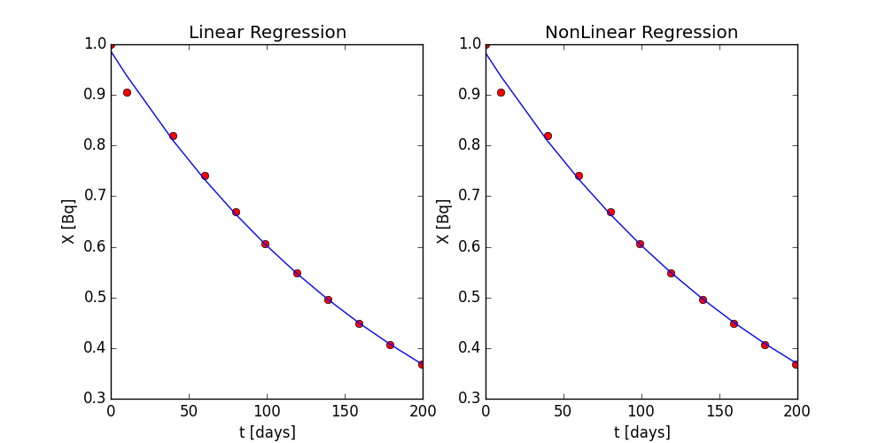
Figure 5: Linear (left) and non-linear (right) regression of the exponential decay data of Polonium-210. The dots are data and the lines are the regression models.
Similar to the analysis of the doubling time in part 4 from Problem 1, the half-life time is also independent of time. The half-life is estimated as
\[{t_h} = – \frac{{\ln \left( 2 \right)}}{a}\]
With this equation, the linear regression predicts a half-life of 140.32 days, and the non-linear regression predicts a half-life of 141.36 days. These are the estimates that are independent from time. If we want to predict when the predicted population will be half of the actual initial condition, we can use the following equation, which is similar from the equation that calculated the doubling time in part 4. The equation is as follows:
\[{t_{{\rm{0}}{\rm{.5}}{{\rm{X}}_f}}} = \frac{1}{a}\ln \left[ {\frac{{0.5{X_i}}}{{X\left( {{t_o}} \right)}}} \right]\]
The linear regression model predicts the time it takes for the initial condition to half is 137.59 days, and the non-linear regression model predicts the time it takes for the initial condition to half is 138.05 days.