Problem 1

Part 1

In the previous module/homework (3), we employed the Euler numerical approximation to solve the Verhulst differential equation. In this module, we will use higher order methods to approximate the numerical solution to improve our accuracy. Because the Verhulst equation has an analytical solution, we can compare each numerical solution to it to evaluate the accuracy. In this module, we will be using multiple functions as well as nested functions. Nested functions are functions within functions. First, we will start with the analytical solution. The analytical solution function can either be inputted with a single condition, to evaluate the population at a certain time (assuming the initial time is zero), or it can be inputted with an array of time to show the evolution of the population. The function is written as follows:

def verhulst_analytical(alpha,K,N_initial,t):
     N = (K * N_initial * np.exp(alpha*t))\
     /(K+N_initial*(np.exp(alpha*t)-1.))
     return N

Next, we required a function that described the time rate of the population (dN/dt) according to the Verhulst equation, where

\[\frac{{dN}}{{dt}} = \alpha N\left( {1 – \frac{N}{K}} \right)\]

def verhulst_rate(N,alpha,K):
     rate = alpha * N * (1.0 - N / K)
     return rate

This function was nested within out numerical schemes. The two schemes that we investigated in this part of the problem was the Euler and 2nd order Runga-Kutta method. The Euler function was as follows:

def euler(Nini,tini,alpha,K,dt,n):
     N = np.zeros((n))
     N[0] = Nini
     for i in xrange(1,n):
          rate = dt * verhulst_rate(N[i-1],alpha,K)
          N[i] = N[i-1] + rate
     return N

This python function models this numerical routine:

\[{N_{new}} = {N_{old}} + \Delta t \cdot f\left( {{N_0},\alpha ,K,{N_{old}}} \right)\]

and the 2nd order Runga-Kutta Method was as follows:

def runga_kutta_2(Nini,tini,alpha,K,dt,n):
     N = np.zeros((n))
     N[0] = Nini
     for i in xrange(1,n):
          k1 = dt * verhulst_rate(N[i-1],alpha,K)
          k2 = dt * verhulst_rate((N[i-1]+k1/2.0),alpha,K)
          N[i] = N[i-1] + k2
     return N

This function models the following numerical routine:

\[\begin{array}{l}{k_1} = \Delta t \cdot f\left( {{N_0},\alpha ,K,{N_{old}}} \right)\\{k_1} = \Delta t \cdot f\left( {{N_0},\alpha ,K,{N_{old}} + {k_1}/2} \right)\\{N_{new}} = {N_{old}} + \Delta t \cdot f\left( {{N_0},\alpha ,K,{N_{old}}} \right)\end{array}\]

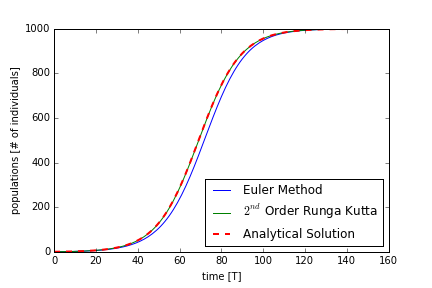
Both the functions, first create the array that the function will output, and then set the initial condition. Using a for loop we iterated the equation in time. The Euler method approximates the differential equation at the (i-1) time step to predict the (i) time step. In a growth model that is fairly exponential, the Euler method will underestimate the derivative of N with respect to t. In contrast, the 2nd order Runga-Kutta method uses the Euler method to approimate a half way point at (i-1/2). At this point, the method makes an additional approximation of the derivative. Using this point, the value of N at time step (i) is found. This method offers a better approximation of the derivative between points at time steps (i-1) and (i). We see in Figure 1 that the 2nd order Runga-Kutta method agrees more with the analytical solution. Figure 1 uses the the following parameters: the growth rate, α = 0.1 days^-1; the time step, dt = 1.0 days; the carrying capacity, K = 1000.0 individuals; and the initial population, N₀ = 1.0 individuals. In Figure 1, we see that the 2nd order Runga-Kutta method more accurately depicts the population evolution than the Euler method. The Euler method systematically underestimates the solution. In the next part, we will employ a Runga-Kutta method with a higher order of accuracy.

Part 2

In this part, we will write a function that uses the 4th order Runga-Kutta numerical method to approximate the solution the the Verhulst population model. The function is as follows:

def runga_kutta_4(Nini,tini,alpha,K,dt,n):
     N = np.zeros((n))
     N[0] = Nini
     for i in xrange(1,n):
          k1 = dt * verhulst_rate(N[i-1],alpha,K)
          k2 = dt * verhulst_rate((N[i-1]+k1/2.0),alpha,K)
          k3 = dt * verhulst_rate((N[i-1]+k2/2.0),alpha,K)
          k4 = dt * verhulst_rate((N[i-1]+k3),alpha,K)
          N[i] = N[i-1] + k1/6.0 + k2/3.0 + k3/3.0 + k4/6.0
return N

This function models the follow numerical routine:

\[\begin{array}{l}{k_1} = \Delta t \cdot f\left( {{N_0},\alpha ,K,{N_{old}}} \right)\\{k_2} = \Delta t \cdot f\left( {{N_0},\alpha ,K,{N_{old}} + {k_1}/2} \right)\\{k_3} = \Delta t \cdot f\left( {{N_0},\alpha ,K,{N_{old}} + {k_2}/2} \right)\\{k_4} = \Delta t \cdot f\left( {{N_0},\alpha ,K,{N_{old}} + {k_3}} \right)\\{N_{new}} = {N_{old}} + \Delta t \cdot f\left( {{N_0},\alpha ,K,{N_{old}}} \right)\end{array}\]

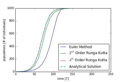
This function takes an weighted sum slope that similar to the 2nd order Runga-Kutta method, but it uses four approximations instead of two. Because it uses more approximations, it is able to more accurately depict the analytical solution. In Figure 1, the 2nd order Runga-Kutta method matched the analytical solution fairly well. To accentuate the differences between the 4th and 2nd order methods, we will increase the time step, dt. This will decrease the accuracy of all of the solutions. We see in Figure 2 that the 4th order Runga-Kutta method agrees more with the analytical solution. Figure 2 uses the the following parameters: the growth rate, α = 0.1 days^-1; the time step, dt = 10.0 days; the carrying capacity, K = 1000.0 individuals; and the initial population, N₀ = 1.0 individuals. Note that the time step is 10 days instead of 1 day. In Figure 2, we see that the Euler is the least accurate, followed by the 2nd order Runga-Kutta method, and then followed by the 4th order Runga-Kutta method. Even with the fairly large value of the time step, the 4th order Runga-Kutta method was able to capture the actual solution well. The errors for the other two methods were that they systematically underestimated the true solution. There is slight overestimation when the population reaches the carrying capacity. Regardless, the estimated time that the numerical solutions took to reach the carrying capacity were similar. This is because the derivative in the beginning of the evolution were underestimated and near the carrying capacity were overestimated. These errors have seemed to cancelled out. When the solution is not near the carrying capacity, the solution usually underestimates the true population. In our previous box model of lake Michigan, because we used the Euler’s method, there may have been unacceptable amount of error. It was not as much as Figure 2 because the time step I personally used was dt = 1 day. Based on this analysis, our Lake Michigan box model could have been improved greatly by either increasing the order of accuracy of our numerical methods or decreasing the time step, dt. For computationally efficiency, it would be much better to change the numerical method.

Problem 2

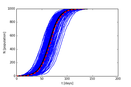
In this problem, we are using a stochastic approach to solving the Verhulst population model. Here we only modeled the integer values of the population and solved for a dt assuming a random value of dN using the equation –ln(1.0 – rnd), where rnd refers to a random number from a uniform distribution from 0 to 1. The equation, –ln(1.0 – rnd), has the expected value of 1. Using this randomly distributed value of dN and a value of N, we can solve for a value of dt. Here we will assume that the time has moved forward at a value of dt, and the population has increased by one. The results are shown in Figure 3. This method relatively efficient to our finite difference approximation because the solution can be vectorized, instead of requiring a for loop. However, this solution requires multiple iterations that are averaged in order to simulate the true solution. As of now, I have trouble understanding the advantages of using this stochastic method for modeling the logisitic growth model. Perhaps it would show its advantages in a more complex growth model. I will think about its applications, and will update this blog if I think of one.