Problem 1
In this problem, we used the python coding language to create a function that could numerically integrate the following equation:
\[f\left( x \right) = a{e^{bx}} + c\]
The code would take inputs of a, b, and c, and find the definite integral between x = 0 and x = 100:
\[\int\limits_0^{100} {\left( {a{e^{bx}} + c} \right)dx} \]
While there are many functions that have no analytical solutions its integral, this one does. Meaning, we can check our numerical approximation of the integral with an analytical solution:
\[\int\limits_0^{100} {\left( {a{e^{bx}} + c} \right)dx} = \frac{a}{b}\left( {{e^{100b}} – {e^{0b}}} \right) + c\left( {100 – 0} \right)\]
I used two different methods for finding the numerical approximation for the integral. The first method was using the library scipy.integrate.quad. This scipy function takes a python function and integrates it between an lower limit and upper limit. The python function contained the equation, which was written as:
def equation(x,a,b,c):
return (a*numpy.exp(b*x))+c
To call the scipy function, we needed to supply the python function’s name, the lower and upper limits, and the additional arguments (a, b, and c). The call looks something like this:
integrate.quad(equation,lower_lim,upper_lim,args=(a,b,c))
where lower_lim is the lower limit and upper_lim is the upper limit. This method gave an estimate that was close to the analytical solution. For example, when a = 1, b = .01, and c = 1, the solution is estimated as 271.828 and the analytical solution is 271.828 (Note: There are many decimals listed, but the numerical solution is accurate to at least 6 decimal points.) As we see, the numerical approximation is very close to the analytical solution.
For completion, the second method was my own. It is a simple trapezoidal approximation of the integral. An additional input that is necessary is a parameter that accounts for the number of cells used for the approximation. The code is as follows:
dx = (upper_lim – lower_lim)/cells
ans = 0.0
for i in xrange(0,cells):
ans = ans + dx/2.0*(equation(dx*i,a,b,c)+equation(dx*(i+1),a,b,c))
where cells is the number of cells. For cells = 10,000, the solution is also 271.828. As cells is decreased the approximation becomes worse. For example, cells = 10 results in a solution of 271.971, which is close, but not as close as the other approximations. The entire code is listed below (Note: I have included it as a image because it is almost impossible to read without the syntax highlighting. Full code is in the supplementary materials page).

Problem 2
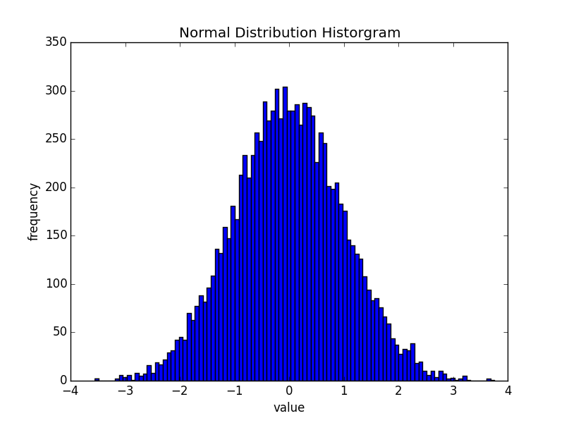
This problem is to write a function that creates a histogram of 10,000 random points that follow a normal distribution. This choice of points are chosen using a mean (avg) and standard deviation (b). The histogram bins (n) the points. The random library was used to choose the points using a normal/gaussian distribution:
for i in xrange(0,num_pts):
x[i] = random.gauss(avg,b)
where x is an array that holds the random values. The histogram was plotted using the histogram function in the matplotlib.pyplot library:
plt.hist(x,bins=n)
Using a standard normal distribution, avg = 0 and b = 1. This creates the following histogram with n = 100.
The code in text format can be found in the supplementary materials page, and here is a screenshot of the code with syntax highlighting.

Problem 3
For this last problem, we writing a function to numerically approximates the volume of 3-sphere. To explain what a 3-sphere is, the following analogy is relevant, Circle : Sphere :: Sphere :: 3-Sphere. It is a sphere in 4D space. A circle’s equation centered at (0,0) is
\[{x^2} + {y^2} = {r^2}\]
where x and y are the dimensions and r is the radius. A sphere’s equation centered at (0,0,0) is
\[{x^2} + {y^2} + {z^2} = {r^2}\]
where z is the third dimension. A 3-sphere’s equation centered at (0,0,0,0) is
\[{w^2} + {x^2} + {y^2} + {z^2} = {r^2}\]
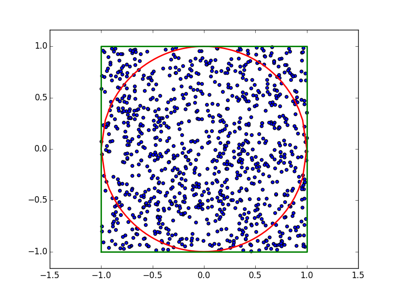
where w is the fourth dimension. The numerical method we will use is called Monte Carlo Integration. This method will be explained using the 2D case, a circle. First, random points using an uniform distribution will be taken from a square of known area (2D volume),
\[4{r^2}\]
Then a circle of radius, r, of 1 will also be added in the center. Since we have an equation for the circle, we know whether the random point is within the circle or not using this inequality:
\[{x^2} + {y^2} \le {r^2}\]
If we know how many points are within the circle and the total number of points, we can use this ratio multiplied by the known area of the square to approximate the area of the circle. Using 1000 points, 781 points we’re within the circle. The approximate volume is then
\[\frac{{781}}{{1000}}{\rm{x}}\left[ {4\left( {{1^2}} \right)} \right]\]
which is 3.124. Using the analytical solution of an area of a circle,
\[\pi {r^2}\]
we know the area is exactly pi.
We can use this same method using the 3-sphere and the inequality:
\[{w^2} + {x^2} + {y^2} + {z^2} \le {r^2}\]
Using 10,000 random points, 3084 points were found within the 3-sphere with r = 5. The volume of the bounding box was
\[{\left( {2r} \right)^4}\]
which is 10,000 in 4D. This makes the volume of the 3-sphere approximately
\[\frac{{3084}}{{10000}}{\rm{x}}\left( {{{10}^4}} \right) = 3084\]
Using the analytical solution of the volume of a 3-sphere,
\[\frac{1}{2}{\pi ^2}{r^4}\]
the volume of a 3-sphere, with r = 5, is 3084.25. The estimation is accurate to the ones place of the analytical solution. More random points will make for a more accurate estimation. Full code can be found in the supplementary material page. The code with syntax highlighting is shown below.
