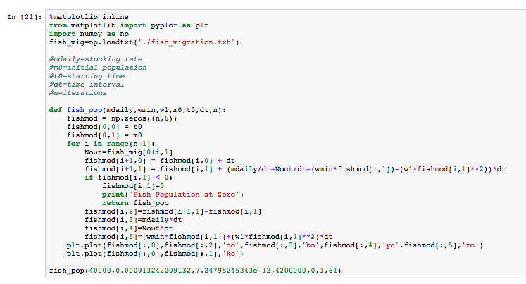
Module 4 consisted of two parts.

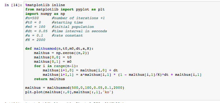
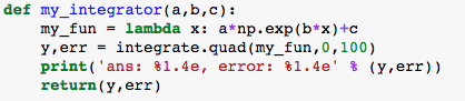
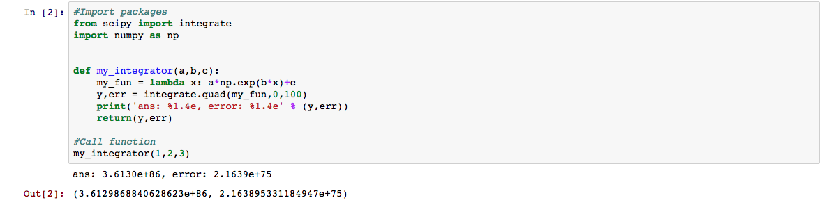
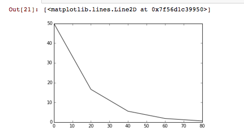
In Mod. 4 Part I, we mainly focused on the finite difference approximation.  In problem 1, I used the Euler’s method nested with the Verhulst equation and a numerical integrator.  We want an analytical method for two reasons.  First, it tells us whether our math is right on the numerical method.  Second, the analytical method tells us our error which is dependent on the time step used.  In Euler’s method, “[steps,2]” was used because for every time step we wanted a row and for every row we want two columns.  My work and the output of both functions is shown below.

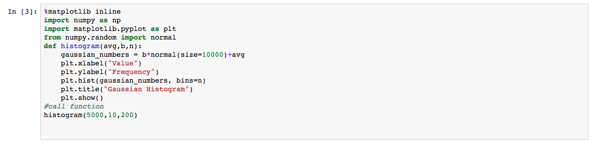
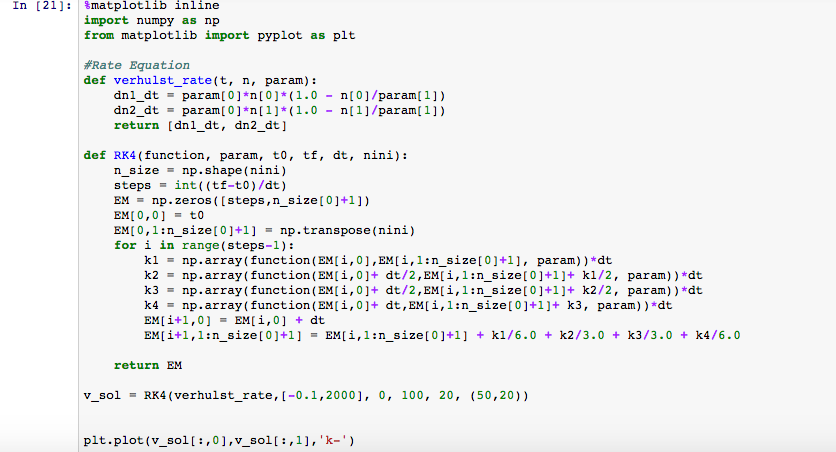
This is the code for part 1, question 1.

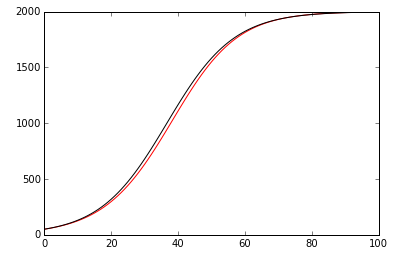
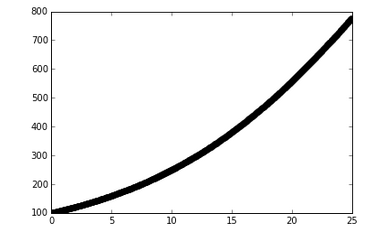
This is the output.

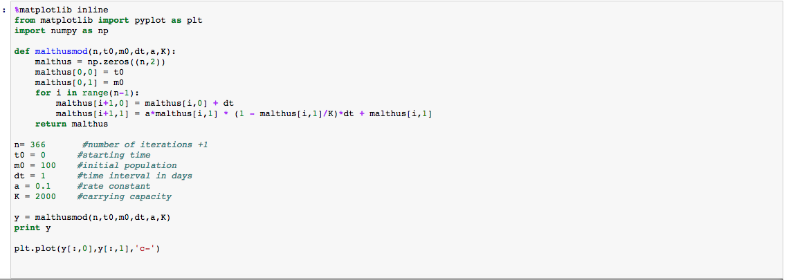
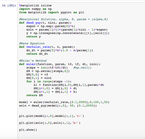
In Module 4 Part II, we had to make a 2 box climate model.  One box represented the temperature of the atmosphere while one box represented the surface temperature.  We used the RK4 code created previously.  See below.

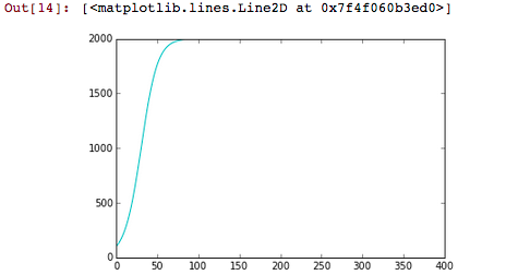
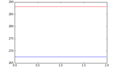
In the second cell, we actually constructed the climate model.  There were several equations and values involved in this process.  We knew that the output of this part should be two flat lines that are stable (i.e. no change occurring).   After looking at all inputs and outputs and correctly modeling them, the resulting code is shown below.  Sure enough, we see two flat lines showing the climate model is in a steady state.

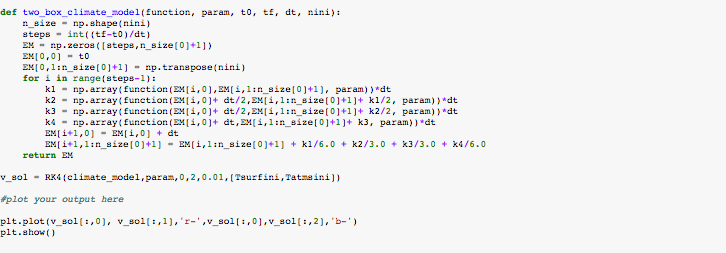
This is the steady state climate model.

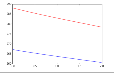
In order to change this steady state, we can manipulate the CO2 and solar input terms.  The first graph shows what happened when I increased the CO2 and solar input values by 50, each.

increased CO2 and solar input

The next graph shows what happened when I decreased the CO2 and solar input values by 50 each.

CO2 and solar input decreased by 50

As you can see, the steady state is no longer maintained when these values are changed.

Problem 1

Our first task in problem 1 was to use the finite difference method to create a population model.  We were given 2 equations and simply had to rearrange Equation 2 and solve for one of the variables, N(t2).  It ended up looking something like this: N(t2) = (t2-t1)((aN(t1)(1-N(t1)/K))+N(t1).

Next, we used the equation above and created a loop in Python from 1 to n.  We use loops when we have code that we want to repeat a fixed amount of times.  My fish population model started with 100 individuals at time = 0, had a rate constant of 0.1, and a carrying capacity of 2000.  This can be seen by my code which I annotated:

This is my code for problem 1 part 2. I named my function “malthusmod” and the values for my conditions may vary from other students.

This is the output from my code. The x-axis indicates days, and the y-axis indicates individuals.

In part 3, I altered the code used above in order to find what day the population reaches 2000 individuals.  As you can see, my last figure did not show that.  My rate constant was changed to 0.1 with 365 iterations (since we wanted to iterate over one year).  The carrying capacity appears to be reached at about 80 days.

For loop to provide us with when the population reaches the carrying capacity of 2000 individuals.

The output of the code above. As you can see, the population stops increasing as the maximum sustainable population is reached.

Problem 2

In this problem, we begin constructing our box model.  This will allow us to look at the number of Coho fish in Lake Michigan throughout a specified time period, in this case, October to early December.  For problem 1, we are given that 5.6 million Coho and Chinook are stocked each year.  Coho represent 3/4 of this number.  The time period that we are dealing with is 3 years, and we are asked for how many fish are stocked per day.

Using the conditions provided, the initial population of Coho and daily stocking rate were found.

In part 2, we are given that 1/3 of the fish population will be migrating during the selected time interval.  We use a histogram to look at the amount of fish that leave each day for 60 days.  The code and resulting figure are shown below:

Code for problem 2 part 2. We were given much of this code and had to fill in some blanks. We also saved data in an external file named “fish_migration”.

The resulting model from the code above. The x-axis represents days, and the y-axis represents individuals.

In part 3, we look at the death rate, which is dependent upon the number of fish in the lake.  This can be shown by Equation 3, which was provided:

I defined my starting minimum rate as the daily stocking rate divided by the initial fish population in Lake Michigan (wmin).  Wmin is density dependent upon the carrying capacity.

Death rate equations

In part 4, we looked at our model over a 30-day time span.  The work up to this point was necessary to get to this step.

The finite difference approximation

The actual model produced by the code above

Problem 1. Regression Analysis of a Population Model

We start off Problem 1 by doing the most basic part of any Python programming, which is importing packages and data.  The outside file “expodata” is being brought in from another file in the same directory.  (Note: skiprows is set to 1 so that you don’t have the words in your data set)

Problem 1 Part 1

Next, we had to write a function for the following expression 

Once again, the first step was to import packages.  The packages that were imported in addition to numpy allow us to see a plot of our data.  I wrote the function itself (called “exponential”) in external file named “expo” (see notes – #Bringing in function from outside file called expo).  We load the data and plot our function to get the following:

Problem 2 Part 2

Part 3 calls for a linear regression.  Once again, we import all necessary packages and our data (expodata).  Then, I linearized the data by using the mathematic function natural log.  We are able to obtain many values from our linear fit, such as the slope, intercept, r value, p value, and standard error.  The data is then converted back to an exponential function which I call “ynew”.  Finally, it is plotted and the data is showed by red circles while the exponential model is a solid black line.

Problem 1 Part 3

Next, we used a nonlinear fit to model our data.  Note that we import the optimize module from scipy in order to do this.  The end product of this allowed me to make a prediction for how long it will take the population to reach its doubled size – about 1.04 years.  However, there may be reasons the colony cannot reach this size; for example, a natural disaster or a predator might change their environment and stop them from reproducing as successfully.

Problem 1 Part 4

Problem 2. Regression Analysis of Chemical Fate Model

In problem 2, we were asked to repeat a lot of what was done in Problem 1 with different data, called “expodata2” this time.  Again, packages were imported and then the data was brought in.  Instead of bringing in an external file, I defined the function normally.  I used the optimize model again to form a nonlinear curve fit.  Some basic algebra was needed in order to rearrange an equation for half life.  The end product gave a half-life value of 141.4 days (since expodata2 used days instead of years) and the end product is shown below.

Problem 2

Problem 2

Problem #1

In Problem 1, we had to write a function in order to solve the following definite integral:

In order to begin this problem, you must import the scipy package for integration.  For this reason, the first line of my code was “from scipy import integrate”.  Next, I imported the numpy package for the exponential component of this problem.  This is written as “import numpy as np” in the second line of my code.

Now we have finished importing all the packages we need to successfully solve this integral.  The next step is to define the function.  We have three variables: a, b, c. Making sure that the function integrates from 0 to 100, defining the function looks like this: 

Finally, we must call the function (the third step to writing any function in python).  This is why the last line of my function reads “my_integrator(1,2,3)”.  The final solution to Homework 1 Problem 1 is shown below.

Problem #2

In Problem 2, we had to create a histogram.  Once again, we followed the same 3 steps to writing any function: import packages, define the function, call the function.

We first had to import the packages matplotlib (in order to see the visual for the histogram) and numpy for the random number generator.  This is why the first 3 lines of my function read:

Now it is time to define the function.  The first part of this reads “def histogram(avg,b,n):” where avg I chose to be 5000, b (the standard deviation) I chose to be 10, and n (the number of bins) I chose to be 200.  For a first timer, I was surprised at how well the histogram looked with these numbers.  The links provided in the description of this problem were very helpful in the second step of this problem which reads: 

Finally, we have to call our function using the values I mentioned above.  The final product of Problem 2 is below [Figure 1].

Figure 1 – Histogram

Problem 2 – final code

Welcome to publish.illinois.edu. This is your first post. Edit or delete it, then start blogging!