Problem 1. Regression Analysis of a Population Model

We start off Problem 1 by doing the most basic part of any Python programming, which is importing packages and data.  The outside file “expodata” is being brought in from another file in the same directory.  (Note: skiprows is set to 1 so that you don’t have the words in your data set)

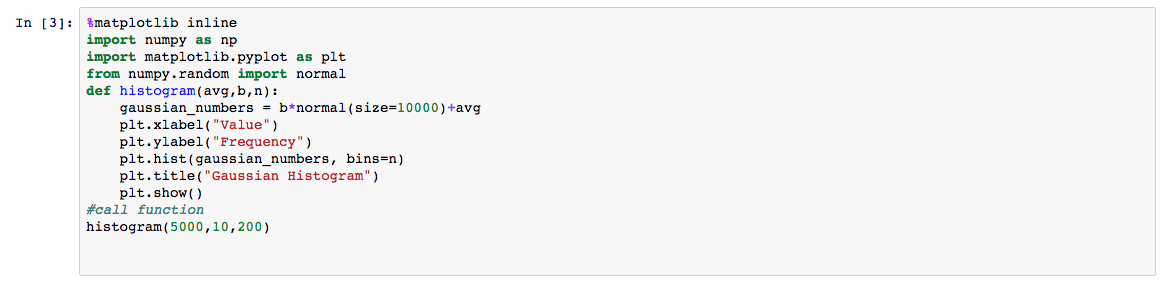
Problem 1 Part 1

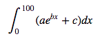
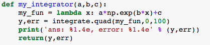
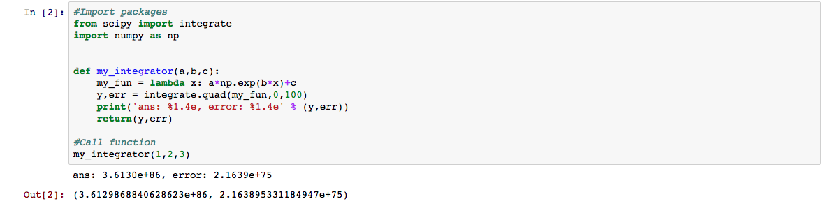
Next, we had to write a function for the following expression 

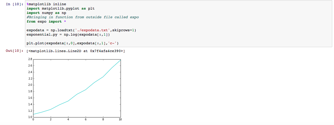
Once again, the first step was to import packages.  The packages that were imported in addition to numpy allow us to see a plot of our data.  I wrote the function itself (called “exponential”) in external file named “expo” (see notes – #Bringing in function from outside file called expo).  We load the data and plot our function to get the following:

Problem 2 Part 2

Part 3 calls for a linear regression.  Once again, we import all necessary packages and our data (expodata).  Then, I linearized the data by using the mathematic function natural log.  We are able to obtain many values from our linear fit, such as the slope, intercept, r value, p value, and standard error.  The data is then converted back to an exponential function which I call “ynew”.  Finally, it is plotted and the data is showed by red circles while the exponential model is a solid black line.

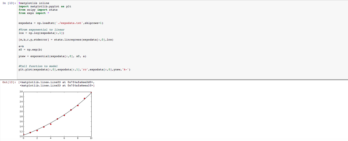
Problem 1 Part 3

Next, we used a nonlinear fit to model our data.  Note that we import the optimize module from scipy in order to do this.  The end product of this allowed me to make a prediction for how long it will take the population to reach its doubled size – about 1.04 years.  However, there may be reasons the colony cannot reach this size; for example, a natural disaster or a predator might change their environment and stop them from reproducing as successfully.

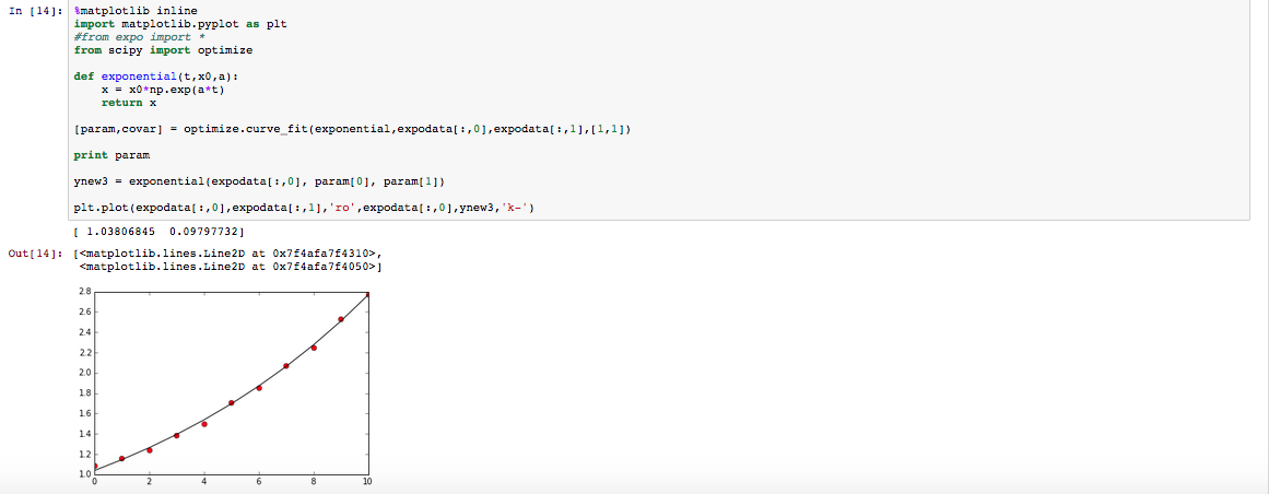
Problem 1 Part 4

Problem 2. Regression Analysis of Chemical Fate Model

In problem 2, we were asked to repeat a lot of what was done in Problem 1 with different data, called “expodata2” this time.  Again, packages were imported and then the data was brought in.  Instead of bringing in an external file, I defined the function normally.  I used the optimize model again to form a nonlinear curve fit.  Some basic algebra was needed in order to rearrange an equation for half life.  The end product gave a half-life value of 141.4 days (since expodata2 used days instead of years) and the end product is shown below.

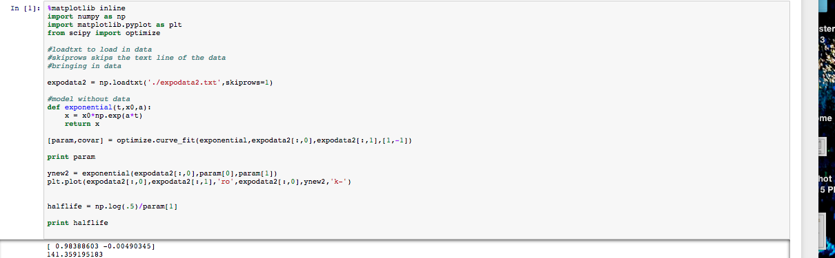
Problem 2

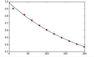
Problem 2

Problem #1

In Problem 1, we had to write a function in order to solve the following definite integral:

In order to begin this problem, you must import the scipy package for integration.  For this reason, the first line of my code was “from scipy import integrate”.  Next, I imported the numpy package for the exponential component of this problem.  This is written as “import numpy as np” in the second line of my code.

Now we have finished importing all the packages we need to successfully solve this integral.  The next step is to define the function.  We have three variables: a, b, c. Making sure that the function integrates from 0 to 100, defining the function looks like this: 

Finally, we must call the function (the third step to writing any function in python).  This is why the last line of my function reads “my_integrator(1,2,3)”.  The final solution to Homework 1 Problem 1 is shown below.

Problem #2

In Problem 2, we had to create a histogram.  Once again, we followed the same 3 steps to writing any function: import packages, define the function, call the function.

We first had to import the packages matplotlib (in order to see the visual for the histogram) and numpy for the random number generator.  This is why the first 3 lines of my function read:

Now it is time to define the function.  The first part of this reads “def histogram(avg,b,n):” where avg I chose to be 5000, b (the standard deviation) I chose to be 10, and n (the number of bins) I chose to be 200.  For a first timer, I was surprised at how well the histogram looked with these numbers.  The links provided in the description of this problem were very helpful in the second step of this problem which reads: 

Finally, we have to call our function using the values I mentioned above.  The final product of Problem 2 is below [Figure 1].

Figure 1 – Histogram

Problem 2 – final code