Computer Vision is used to solve an interesting problem in Robotics, which has applications in navigation of unknown places and territories.
This area is known as SLAM, or Simultaneous Localisation and Mapping. Essentially, the problem that SLAM attempts to solve is “How can a robot create a map of its surroundings and localise itself in the map its created by itself?”. The solutions for this problem will allow a robot to navigate a terrain autonomously, without the use of external navigation sources, such as GPS.
There are several implementations of simulations of SLAM methods available online. I decided to attempt to reproduce the results of a paper issued by a university in Germany. The link to their webpage is available here: http://vision.in.tum.de/research/quadcopter.
INSTALLATION:
In order to implement my system, I had to install several packages, and run some libraries in Linux.
I plan to create a simulation using the package gazebo. Gazebo is a popular simulation used to model robots.
After installing all the packages, I was able to run the simulation that was provided in the package.
I decided to use a tutorial available at this website: http://wiki.ros.org/hector_quadrotor/Tutorials/Quadrotor%20indoor%20SLAM%20demo
Implementing a complete SLAM system was a larger task than expected. Since this project required a significant portion completed by myself, it was difficult to find a paper which did not use a large number of external libraries. This made it difficult for me to use a paper to implement something by myself. For this reason, I have decided to focus on special topic within SLAM; Object tracking.
Through this project, I will attempt to implement an algorithm in Matlab, to detect moving objects in a scene. The algorithm will incorporate some code from previous projects, such as the auto_homography function. In essence, this is an extension of Project 5.
IMPLEMENTATION:
Task 1:Setting up the framework
I decided to use Matlab, as I was most comfortable with this software, and this project made use of several matrix calculations.
Task 2: Create a model to work with;the dual-Jacobian visual interaction model
According to the paper, an equation can be created to model the system. The following equation is a model of the velocity of the robot.
![]() [3]
[3]
The same paper has a very useful figure to illustrate this:
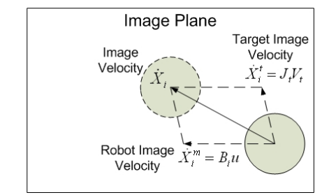 [3]
[3]
In this equation, the Jt and Bi represent matrixes with matrixes that depend on angles and positions of the objects. The “JtVt” term is connected to the position and velocity of the objects in a frame. The “Biu” term is connected to the velocity of the robot that is recording the visual data. If our robot is stationary, then this term goes to 0.
Task 3: Building upon the previous code for prior projects
I used the autohomography script, provided in Project 5, and altered it to provide useful output for this project.
I altered the try_correspondance to output the distance between objects at two positions, as seen in this example done with started code from Project 5.
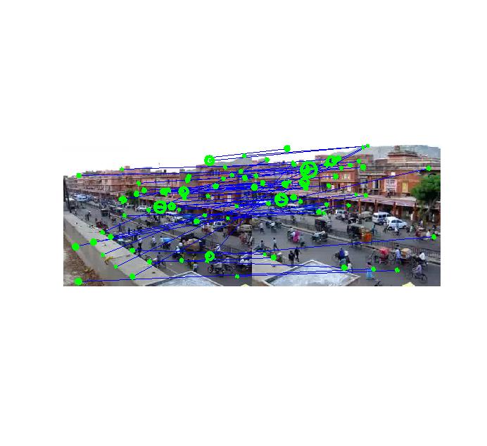
I calculated the difference between the x positions and y positions in these images,
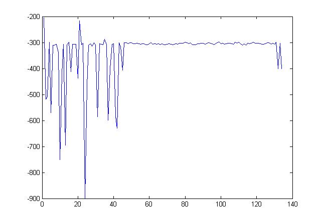
(plot of differences in values of x position from all objects)
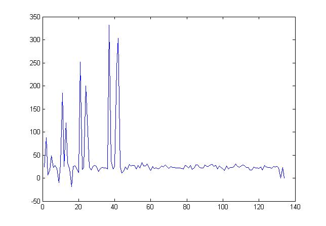
(plot of differences in y position from all objects)
These graphs are important because there is a region which is fairly constant. This value represents the average change in position of the objects in this scene. In this example, the average values come out to be
x= -310.54 and y= 17.33
This value can be used to replace the position terms in the “JtVt” directly. I am going to check if this value can be used to compute the position of the robot.
However the velocity is still unknown.
Task 4: Kalman filter
As part of this paper, a Kalman filter was required to be created. I used the equations in the paper to create some calculations. My graph came out very strange.
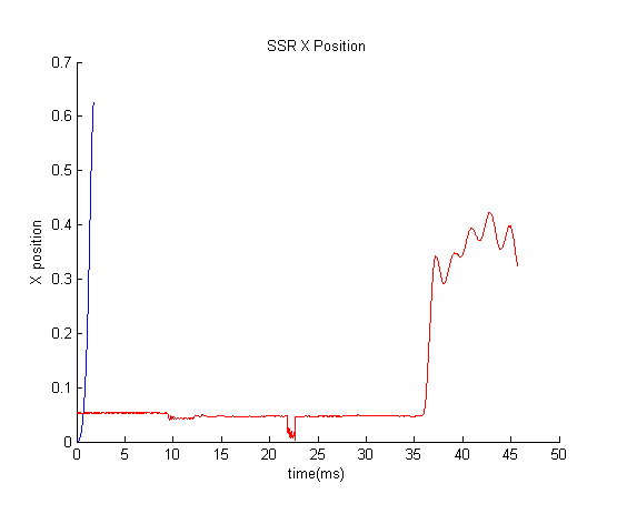
The red graph was a vector that I used to test the Kalmann filter. There is noise from about 36 milliseconds. I expected my Kalman filter(the blue line) to create a line of constant x position, however somehow my Kalmann filter somehow went to a high value in the initial milliseconds.
This error could potentially come from a mistake in my implementation of the filter.
Task 5: Establishing communication with simulation
The Matlab program was run on a Windows machine, and the results were computed in Matlab as well.
In order to show the results, a live demonstration could be used. However, due to my limited knowledge of hardware issues involved in connecting the AR drone to my Matlab program, I decided to try to create a simulation which used values computed in Matlab.
The Gazebo simulator was the simulator of choice. Along with a package in ROS called hector_quadrotor(available at http://wiki.ros.org/hector_quadrotor), I tried to replicate the results shown in this simulation:
In order to use the simulator, I had to install several packages. These included :
1) gazebo(the simulator)
2)rviz(the visual platform to view the final animations)
3) joy_node(for joystick control, although the terminal could also be used)
4)ardrone_autonomy(official driver for AR Drone flying robots)
5)tum_simulator(a simulator developed by TUM University)
PROBLEMS FACED
In implementing the SLAM simulation, I faced several issues that prevented me from successfully completing all the objectives of my project.
- Gazebo-Matlab communication – Since I was a beginner to Gazebo, I used a library that was supposed to establish communication between Matlab and Gazebo. However, there were several compile errors, which I could not resolve even after several hours of trial and error. This prevented me from improving my simulation, and creating a demo where data from Matlab could be used as input to move the robot simulation in real time.
- AR Drone hardware issues- I planned to implement a live demo, where I could use a drone to navigate using markers it used from its camera. However, the drone did not seem to respond to the signals sent online. It was also difficult to connect the Matlab program from my computer to the drone wirelessly. With a wire, although the data could be transmitted, the drone was limited in flying range due to the length of the wire.
- The Kalman filter used to implement the calculation to find the values of velocity and position provided strange graphs, which suggest a mistake on my part as to how I implemented the formula provided on the paper.
REFERENCES:
- http://www.robots.ox.ac.uk/~gk/publications/KleinMurray2007ISMAR.pdf
- http://www.cs.berkeley.edu/~pabbeel/cs287-fa09/readings/Durrant-Whyte_Bailey_SLAM-tutorial-I.pdf
- Robust Mobile Robot Visual Tracking Control System
Using Self-Tuning Kalman Filter,Chi-Yi Tsai, Kai-Tai So,Dutoit, Hendrik Van Brussel ,Marnix Nuttin,2007 IEEE International Symposium,June 20-23
(http://ieeexplore.ieee.org/stamp/stamp.jsp?tp=&arnumber=4269860&tag=1)