Authors: Ashwathi Iyer and Yubo “Paul” Yang
Stability of Water Between Graphene Sheets
INTRODUCTION
The importance of water cannot be downplayed. Bulk water runs in oceans, lakes and even our very own bodies. It is a crucial ingredient in photosynthesis and can act as lubricant in many biological and even geological processes. Its solid form is even more fascinating, as it varies in structure and property. Ice is of crucial importance in many fields ranging from material science to biology. Despite the large amounts of experimental and theoretical studies on various phases of water, many of its properties remain elusive. In particular, uncertainties remain on various ground state structures of ice in its phase diagram. Most ice structures are locally tetrahedral. This is true even in the amorphous phases and in the so-called cubic-ice phase (Ic). Interestingly, experiments have shown that the local tetrahedral environment may be broken for confined ice. In particular, we are fascinated by a recent experimental observation that ice can form a simple cubic lattice in between layers of graphene.
SUMMARY OF RESULTS
- We simulated a monolayer and bilayer of water between graphene sheets at quarter and full coverages using DFT and CPMD
- We observe square ice at quarter coverage
- For bilayer, we observe a transition to square ice at 1.5 GPa
- We observe that ice prefers a triangular or disordered structure with local tetrahedral coordination at full coverage
- We also implemented a CPMD code for a hydrogen atom and present its ability to do energy minimization based on the concept of simulated annealing
METHOD: CPMD
One challenging aspect in the study of ice is the proper treatment of the proton motion. Due to the prevalence of hydrogen bonds in ice, the quantum nature of the proton must be considered. While an appropriately parametrized forcefield may be able to capture many aspects of these quantum effects, a fully ab initio study is needed for an accurate treatment without a priori assumptions.
Types of Ab-Initio Molecular Dynamics
1. Ehrenfest MD
- Electronic Hamiltonian depends parametrically on classical nuclear positions
- Nuclei are treated as classical particles, while electrons are treated quantum mechanically
- Nuclear degrees of freedom: Evolve through classical equations of motion
- Electronic degrees of freedom: Evolve through the Schrodinger equation
2. Born-Oppenheimer Molecular Dynamics
- Ensure wavefunction at each timestep is the ground state adiabatic wavefunction
- Allow nuclei to move on this ground-state Born Oppenheimer potential energy surface and obtain forces through the Hellman-Feynman theorem
- Good approximation when energy difference between ground and first excited state is much smaller than kT
- But need to solve the electronic problem at every time step 🙁
3. Carr-Parrinello Molecular Dynamics
- Avoids solving the the electronic (DFT) problem at every time step by realizing that there are two timescales in the problem: fast (quantum) electronic motion and slow (classical) nuclear motion
- Perform a single DFT calculation to obtain the Kohn-Sham orbitals near the ground state
- Shift to a purely classical problem by constructing a Lagrangian that parametrically depends on the nuclear coordinates and the Kohn-Sham orbitals
- Forces on nuclei: Derivative of Lagrangian with respect to the nuclear coordinates
- Forces on orbitals: Derivate of Lagrangian with respect to orbitals
CPMD is conceptually very straight-forward to understand from a simulated annealing perspective. Simulated annealing is a general minimization procedure that works as long as an objective function can be calculated given a set of variables. Here Kohn-Sham energy functional is the objective function and nuclear coordinates, electronic orbital coefficients and environmental constraints are the variables. Lagrangian dynamics is just one way to perform such minimization. As we evolve variables with the equations of motion designated by the chosen Lagrangian, we simulate the dynamics of the ions while keeping the electronic orbital in its ground state. This is analogous to evolving the ions on the ground state Born-Oppenheimer potential surface (with an appropriate choice of Lagrangian). The fascinating part is that with a “good” choice of the Lagrangian, the dynamics of the ions are actually physical!
SIMULATION SETUP
Sanity Check: Monolayer of water on a single graphene sheet
Monolayer of water on a single graphene sheet is unstable as graphene is hydrophobic in its natural state.
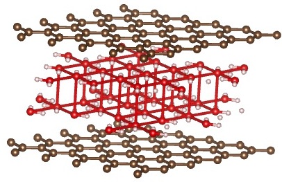
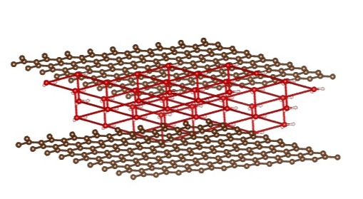
A layer of water sandwiched between 2 graphene sheets
Sideview of water sandwiched between graphene sheets
Simulation Parameters
Software packages used:
VASP & Quantum Espresso (simulation)
VESTA, xcrysden (visualization)
| Quarter Coverage | Full Coverage |
|---|---|
| 64 C atoms, 4 H2O molecules | 64 C atoms, 16 H2O molecules |
Simulation Parameters
| Plane wave cutoff | 520 eV |
| Fictitious electron mass | 100 a.u. |
| Time step | 4.84E-17 s |
| Number of simulation steps | 10000 |
RESULTS
Outline
We looked at 4 setups:
- Quarter coverage, monolayer (Square, Triangular)
- Full coverage, monolayer (Square, Triangular)
- Full coverage, bilayer (Square, AA/AB Stacking)
- Quarter coverage, bilayer (Square, AA/AB Stacking)
Quarter Coverage: Monolayer of Water
Energy difference from DFT: 3.94 eV (Square ice configuration is more stable)
Energy from CPMD: 6.5(3) eV (Square ice configuration is more stable)
Square ice structure is more stable in both cases.
| Pressure (GPa) | 0 | 1.0 |
|---|---|---|
| Enthalpy Difference (eV) | 6.64(2) | 6.5(3) |
CPMD calculations performed at 0 GPa, 0.5 GPa and 1.0 GPa all show the same qualitative difference. Therefore the square ice structure is more stable than the triangular ice structure as a monolayer. Our results at low coverage agree with those in the paper.
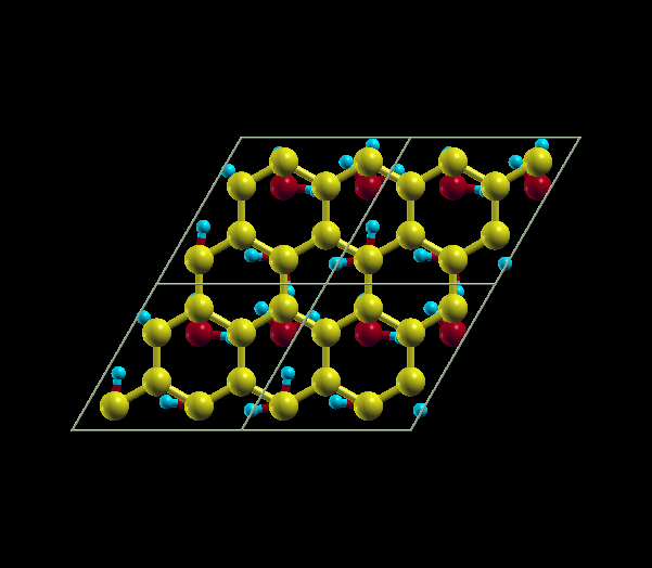
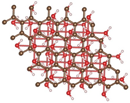
Full Coverage: Monolayer of Water
Ice prefers a triangular lattice instead of a square lattice! Structural relaxation using DFT relaxes to a triangular structure when the initial structure is square.
| E(triangular) - E(square) | |
|---|---|
| DFT | 5.8 eV |
| CPMD | 0.064 eV |
CPMD simulation with triangular lattice and square lattice as initial configuration shows the triangular lattice is more stable, but the square lattice did not change its configuration during the run. This could be because the timescale needed to observe a lattice reorganization is way beyond the accessible timescale on the femto second scale.
Full Coverage: Bilayer of Water
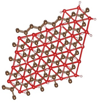
Here, instead of starting in square and triangular configurations, we start in a square configuration, but with AA and AB stacking of the water molecules, arranged in a cubic lattice.
We get very different results from the paper. When starting with AA stacking, the cubic lattice rearranges itself into a triangular lattice, as it did in the case of a single layer of water.
Initial structure – AA stacking, Cubic Lattice
↓
Final Structure – AA Stacking, Triangular Lattice
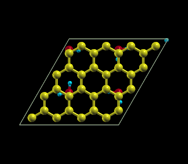
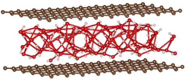
When starting with AB stacking, the water molecules relax to a structure that has no in-plane order, but maintains local tetrahedral coordination. This structure is more stable by ~ 7.9 eV.
AB stacking, cubic lattice (initial) → AB stacking, final relaxed structure
Quarter Coverage: Bilayer of Water
- Let’s see what happens with a bilayer of water at quarter coverage
- Presumably Van der Waals interactions are weaker now
Energy (AA Stacking) > Energy (AB Stacking) (Δ E = 0.128 eV)
- AB stacking disorders below 1.5 GPa!
- But @ 1.5 GPa and higher: AB stacking is in a square lattice
AB Stacking Side view: AB Stacking
DISCUSSION OF RESULTS
Our results are in good agreement with the Nature article at low coverage but not at high coverage!
- Possible origin: Van der Waals forces between water molecules?
- At low coverage, Van der Waals interactions are weak ⇒ Might be possible to recover result in the Nature article
- But expected a higher transition pressure (1.5 GPa) because water molecules in our simulation are much farther away than they are in the paper
- Van der Waals interactions are not captured by DFT/CPMD
- Indication that observed square/cubic lattice not a result of including dynamics
- Explains why the paper uses an empirical force field and classical MD
IMPLEMENTATION OF CPMD FOR A TOY SYSTEM
We have implemented a CPMD code for a hydrogen atom using periodic boundary conditions. Our code consists of two parts:
- A plane wave DFT code that minimizes the electronic orbitals to the electronic ground state
- An MD code that simulates dynamics on the ion and electron orbitals, including an implementation of the SHAKE algorithm to maintain the constraint of orthonormality of orbitals
The code is on Github for those interested.
Ion Dynamics
When we start a CPMD simulation close to the electronic ground state and with the ion moved slightly away from the known ground state position, we observe that the ion is pushed back to the center.
Relationship to Simulated Annealing
To demonstrate the CP method’s ability to solve for the electronic ground state wave function, we use an initial guess for the ground state coefficients that is perturbed from those of the true ground state by a random vector. Then we evolve the electronic degrees of freedom keeping the ions fixed. This effectively minimizes the Kohn-Sham energy function through a simulated annealing procedure which should reproduce the ground state eigenvalue and eigenvector obtained using DFT.
Once the wave function is expanded in the plane wave basis, the Kohn-Sham energy function becomes nothing more than a multivariable function of the expansion coefficients
\(\psi(\vec{r})=\sum\limits_{i=1}^{N_b} c_{i} \left( \frac{1}{\sqrt{V}} e^{i\vec{k}_i\cdot\vec{r}} \right) \Rightarrow E[\psi] = E(\{c_i\})\)
The ground state coefficients can be obtained by minimizing the energy with the normalization constraint
\(g=\int \vert\psi(\vec{r})\vert^2d\vec{r}-1=0 \)
In classical simulated annealing, we traverse the phase space with Metropolis moves, here we use a Lagrangian
\(\mathcal{L} =\frac{1}{2}\mu \int \vert\dot{\psi}(\vec{r})\vert^2d\vec{r} – E[\psi]+\lambda\int\vert\psi(\vec{r})\vert^2d\vec{r} \)
Energy Trace Norm of Orbital Time Step Convergence
CONCLUSIONS
- We simulated a monolayer and bilayer of water between two sheets of graphene, at quarter coverage and full coverage
- The ground state is a square or cubic ice structure at low coverage
- The ground state is triangular or disordered (with local tetrahedral coordination) at higher coverage.
- We reason that this might be a result of the strong Van der Waals interactions between water molecules that are not captured by CPMD or DFT calculations.
- We also conclude that our results suggest that the dynamics of the water molecules don’t necessarily play a huge role in square ice formation between graphene sheets.
- We also implemented a CPMD code for hydrogen
- We demonstrate energy minimization using the simulated annealing interpretation of CPMD and show that this is effectively equivalent to a Hartree-Fock approach.
FURTHER READING
1) CPMD code
2) Final Report