The box model describes the continuity equation which holds varying rate components (constantly monitored) that collectively make up a system as a whole. An extension of the single box model is a two box model which serve as two systems co-existing in the same environment. The co-existing systems represent two quantities that we wish to track simultaneously to see how it affects a main system. A typical example of this model is the global climate system. This system uses quantitative forms to simulate solar energy interactions in the environment. The energy interactions regulate the atmospheric temperatures as well as the earth’s surface temperatures and these two variables conjointly control the global climate .
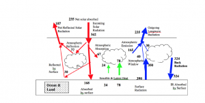
Figure 1: Diagram of energy sources and sinks of radiation contributing to climate
The co-existing systems shown in the climate model route the incoming and outgoing solar radiation in two separate cycles to cause a balance in the earth’s incoming and outgoing energy flows. The solar radiation in each cycle is reflected, absorbed, chemically stored by photosynthesis, before been emitted back beyond the earth’s atmosphere. These changes in energy forms have been incorporated into the model to bring about an overall change in the climate system.
This exercise interestingly reviews factors that affect global temperatures such as solar insolation, reflection , cloud cover, green house gases and so on. The factors are expressed in mathematical forms and built into the Rung-Kutta integrator to obtain the most realistic and credible model. Once the model is built at standard conditions, the factors are altered to see how it influences global temperatures and this is seen by the model’s responsiveness.
Experimentation with the Two Box Climate Model
Constructing the 2-box Climate Model
The first step is to build the model at temperatures that maintain it at equilibrium for perpetuity. These temperatures are actually the base values used for the iteration. They are set at 288.99K and 267.44K and these represent the initial surface temperature and atmospheric temperature respectively. In addition, the co-existing systems are built into the model as thermal reservoirs to enable us account for the energy flows. The two reservoirs are the atmospheric (energy source) and earth’s surface (energy sink) reservoirs which primarily includes the oceans. The energy source reservoir increases the energy rate in the climate system while the energy sink reservoir decreases or absorbs energy from the system. Both reservoirs interact to balance the climate system.
As built into the model, the surface reservoir (energy source) contains the following equations:
i.) Energy inflow from the sun to the earth’s surface
![]() …..eqn 1
…..eqn 1
![]() ……..eqn 2
……..eqn 2
ii.) Energy inflow by atmospheric input into the earth’s surface
![]() …eqn 3
…eqn 3
![]() … eqn 4
… eqn 4
![]() … eqn 5
… eqn 5
iii.) Energy outflow emitted by the earth’s surface
![]() ….eqn 6
….eqn 6
![]() ….eqn 7
….eqn 7
The atmospheric reservoir contains the following equations:
iv.) Energy inflow from the sun to the earth’s atmosphere
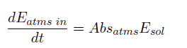 … eqn 8
![]() …eqn 9
…eqn 9
v.) Energy outflow from the atmospheric sink and a surface source
![]() …eqn 10
…eqn 10
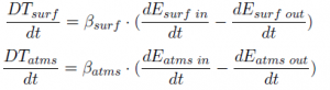
The equations above are used in computing the infinitesimal changes in temperatures with respect to time. These values are included in the iterations to obtain increasing magnitudes of the base temperature.
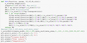
Using aforelisted equations with a preset carbon dioxide level of 320ppm, water vapor rate of 1 , solar insolation of 342 W/m2, time step of 0.001 and an ocean mixed layer depth of 50; the algorithm and resulting model at equilibrium is shown below as:

a.) Altering Solar Input – Investigating the Response Time and Sensitivity
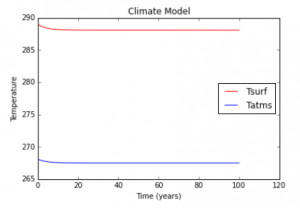
In this experiment, we investigate how sensitive the climate system is in responding to changes in the solar energy received by Earth. The average amount of radiation emitted by the sun is 342W/m2. By changing the solar insolation by 3% at each run for three consecutive years, we see the effect on surface and atmospheric temperatures.
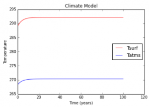
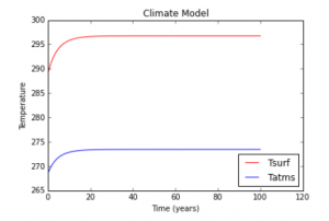

The three figures represent the climate model at solar insolation levels of 352.26W/m2, 362.83W/m2 and 373.71W/m2 respectively. From the graph plots, we observe an increase in the surface and atmospheric temperatures as solar insolation increases.
b.) Altering Cloud Cover
This model proves that cloud cover is dependent on surface temperature. At the surface temperature set to maintain equilibrium (288K), 60% if the earth surface is covered by clouds. To see the effect of cloud cover on the climate system, we use the values listed in the table below.
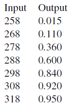
The output column in the table above represents the degree of coverage in decimals. For example, at 288K, the earth surface is covered by 60% clouds. By modifying the algorithm displayed above using these values, the resulting effect on the model is shown below as:

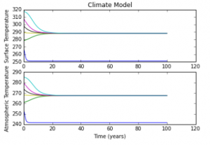
The highest surface temperature (320K) in the model reflects the greatest amount of cloud cover and vice versa. Plot 1 and 2 shows the resultant effect of cloud cover on surface and atmospheric temperatures. For all temperatures above 290K in plot 1, we observe a gradual decrease in temperatures until the system reaches equilibrium. This explains how a higher volume of clouds would reflect a larger amount of solar insolation thereby reducing surface temperatures. The same explanation applies for temperatures above 270K in plot 2. The model predicts that temperature would rise with less cloud cover and fall when there is a large amount of cloud cover. However, the surface and atmospheric temperatures cannot go beyond 290K and 270K after 20years.
c.) Removing Greenhouse Gases
Greenhouse gases absorb reflected infrared radiation and trap the heat in the atmosphere thereby warming the earth . They increase in global temperatures can lead to a chain of events such as increased rainfall, rise in sea level ,greater risk of drought, more heat waves and so on. The main greenhouse gases accounted for in this model are (water vapor (H20) and carbon dioxide CO2). By removing the energy emitted by land that is absorbed into the atmosphere, we can get rid of the greenhouse gases. This is effected in the model by setting EMSatms (eqn 3) to zero and this generates resulting effect shown in the figure below.
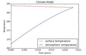
Removing these greenhouse gases from the atmosphere, reduces the amount of heat trapped in the atmosphere. This is evident in graph by the slight decrease of surface temperatures however, the atmospheric temperature rises till it reaches the same point as the surface temperature.
d.) Enhancing the Greenhouse Effect
The model predicts the likely effects of increasing and decreasing the level of greenhouse gases in the atmosphere. The model is tested at different concentrations of CO2 and H20 in the atmosphere. The results interestingly reveal the following:
a.)  b.)
b.) 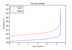
c.) 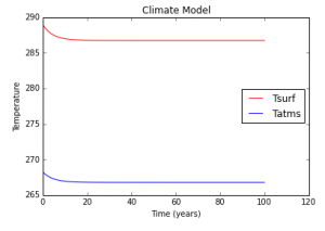 d.)
d.) 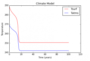 The four graph plots represent:
a.) The effect on the climate system when CO2 concentration is doubled
b.) The effect on the climate system when CO2 and H20 concentration are doubled.
c.) The effect on the climate system when CO2 concentration is halved.
d) The effect on the climate system when CO2 and H20 concentration are halved
By doubling the concentration of CO2 in the atmosphere, we observe a slight increase in both surface and atmospheric temperatures. Scientists predict that the earth’s temperature would increase by 1 degree centigrade if the concentration of CO2 is doubled, and this estimate is confirmed in the model.
Plot (b) shows that H20 is a very dominant greenhouse gas. When the concentration of CO2 and H20 are doubled simultaneously, the climate system experiences a gradual increase in temperatures until it climbs drastically after 5 years. Plot (c) and (d) show expected changes in temperatures when the concentration of the greenhouse gases are halved. This demonstration proves that the greenhouse gases have a strong effect on the climate system and could lead to unpleasant consequences if the gases are not regulated.