A Different Kind of Data Cleaning: Making Your Data Visualizations Accessible

Introduction: Why Does Accessibility Matter?

Data visualizations are a fast and effective manner for communicating information and are increasingly becoming a more popular way for researchers to share their data with a broad audience. Because of this rising importance, it is also necessary to ensure that data visualizations are accessible to everyone. Accessible data visualizations not only help an audience who may require a screen reader or other accessible tool to read a document but are also helpful to the creators of the data visualization as it brings their data to a much wider audience than through a non-accessible data visualization. This post will offer three tips on how you can make your visualization accessible!

TIP #1: Color Selection

One of the most important choices when making a data visualization are the colors used in the chart. One suggestion would be to use a color blindness simulator to check the colors in the data visualization and experiment to find the right amount of contrast between colors. Look at the example regarding the top ice cream flavors:

A data visualization about the top flavors of ice cream. Chocolate was the top flavor (40%) followed by Vanilla (30%), Strawberry (20%), and Other (10%).

At first glance, these colors may seem acceptable to use for this kind of data. But when ran through the colorblindness simulator, one of the results creates an accessibility concern:

This is the same pie chart above, but placed under a tritanopia color blindness lens. The colors used for strawberry and vanilla now look the exact same and blend into one another because of this, making it harder to discern the amount of space they take in the pie chart.

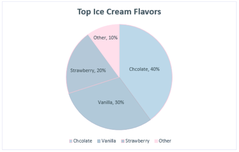
Although the colors contrasted well enough in the normal view, the color palettes used for the strawberry and vanilla categories look the same for those with tritanopia color blindness. The result is that these sections blend into one another and make it more difficult to distinguish their values. Most color palettes incorporated in current data visualization software are already designed to ensure the colors do not contrast, but it is still a good practice to check to ensure the colors do not blend in with one another!

TIP #2: Adding Alt Text

Since most data visualizations often appear as images in either published work or reports, alt text is a crucial need for accessibility purposes. Take the visualization below. If there was no alt text provided, then the visualization is meaningless to those who rely on alt text to read a given document. Alt text should be short and summarize the key takeaways from the data (there is no need to describe each individual point, but it should provide enough information to describe the trends occurring in the data).

This is a chart showing the population size of each town in a given county. Towns are labeled A-E and continue to grow in population size as they go down the alphabet (town A has 1,000 people while town E has 100,000 people).

TIP #3: Clearly Labeling Your Data

A simple but crucial component of any visualization is having clear labels on your data. Let’s look at two examples to see what makes having labels a vital aspect of any data visualization:

This is a chart for how much money was earned/spent at a lemonade stand by month. There is no y-axis labels to describe how much money is earned/spent and no key to discern the two lines that represent the money made and the money spent.

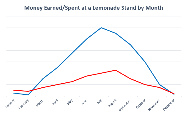
There is nothing in this graph that provides any useful information regarding the money earned or spent at the lemonade stand. How much money was earned or spent each month? What do these two lines represent? Now, look at a more clearly labeled version of the same data:

This is a cleaned version of the previous visualization regarding how much money was earned/spent at a lemonade stand. The addition of a Y-axis and key now show that more money was spent in January/February than earned, but then changes in March peaking in July, and then continuing to fall until December where more money is spent than earned again.

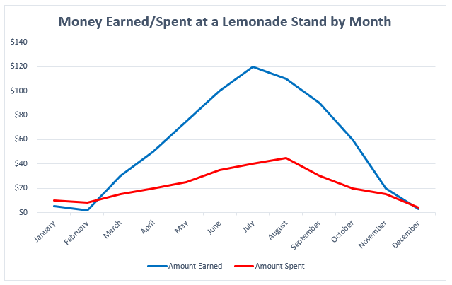
In adding a labeled Y-axis, we can now quantify the difference in distance between the two lines at any point and have a better idea of the money earned/spent in any given month. Furthermore, the addition of a key at the bottom of the visualization distinguishes the lines telling the audience what each represents. By clearly labeling the data, it is now in a position where audience members can interpret and analyze it properly.

Conclusion: Can My Data Still be Visually Appealing?

While it may appear that some of these recommendations detract from the creative designs of data visualizations, this is not the case at all. Designing a visually appealing data visualization is another crucial aspect of data visualization and should be heavily considered when creating one. Accessibility concerns, however, should have priority over the visual appeal of the data visualization. That said, accessibility in many respects encourages creativity in the design, as it makes the creator carefully consider how they want to present their data in a way that is both accessible and visually appealing. Thus, accessibility makes for a more creative and transmissive data visualization and will benefit everyone!

Scary Research to Share in the Dark: A Halloween-Themed Roundup

If you’re anything like us here in the Scholarly Commons, the day you’ve been waiting for is finally here. It’s time to put on a costume, eat too much candy, and celebrate all things spooky. That’s right, folks. It’s Halloween and we couldn’t be happier!

Man in all black with a jack o' lantern mask dancing in front of a green screen cemetery

If you’ve been keeping up with our Twitter (@ScholCommons) this month, you’ve noticed we’ve been sharing some ghoulish graphs and other scary scholarship. To keep the holiday spirit(s) high, I wanted to use this week’s blog post to gather up all our favorites.

First up, check out the most haunted cities in the US on The Next Web, which includes some graphs but also a heat map of the most haunted areas in the country. Which region do you think has the most ghosts?

If you’re more interested in what’s happening on across the pond, we’ve got you covered. Click on this project to see just how scary ArcGIS story maps can be.

https://twitter.com/ScholCommons/status/1187058855282462721

And while ghosts may be cool, we all know the best Halloween characters are all witches. Check out this fascinating project from The University of Edinburgh that explores real, historic witch hunts in Scotland.

The next project we want to show you might be one of the scariest. I was absolutely horrified to find out that Illinois’ most popular Halloween candy is Jolly Ranchers. If you’re expecting trick-or-treaters tonight, please think of the children and reconsider your candy offerings.

Now that we’ve share the most macabre maps around, let’s shift our focus to the future. Nathan Yau uses data to predict when your death will occur. And if this isn’t enough to terrify you, try his tool to predict how you’ll die.

Finally, if you’re looking for some cooking help from an AI or a Great Old One, check out this neural network dubbed “Cooking with Cthulhu.”

Do you have any favorite Halloween-themed research projects? If so, please share it with us here or on Twitter. And if you’re interested in doing your own deadly digital scholarship, feel free to reach out to the Scholarly Commons to learn how to get started or get help on your current work. Remember, in the words everyone’s favorite two-faced mayor…

A clip of the Mayor from Nightmare Before Christmas saying There's only 365 days left until next Halloween

Exploring Data Visualization #10

In this monthly series, I share a combination of cool data visualizations, useful tools and resources, and other visualization miscellany. The field of data visualization is full of experts who publish insights in books and on blogs, and I’ll be using this series to introduce you to a few of them. You can find previous posts by looking at the Exploring Data Visualization tag.

A collage of images of sticky notes in different configurations from the article "stickies!"

Sticky notes in all different shapes, sizes, and colors provide a perfect medium for project planning.

1. Sometimes when you want to visualize your thinking, digital tools just don’t cut it and you have to go back to cold, hard paper. At the beginning of November, Cole Nussbaumer Knaflic at Storytelling with Data made a #SWDchallenge for readers to use sticky notes to represent their thinking and plan out a data visualization the old fashioned way! The images that resulted from that challenge, seen in the post stickies!, are an office-supply lover’s dream. I’ve taken inspiration from these posts in my own project planning for the past month—here’s a sneak peek of my thoughts for a sign that will be displayed in a library study space:

A piece of paper that reads "Welcome to Room 220" at the top with sticky notes stuck to the page underneath.

2. In a feature from February of this year, the digital branch of German newspaper Die Zeit, ZEIT ONLINE, showed some interesting finds from their database of approximately 450,000 street names used across Germany. They call the project Streetscapes and use them to explore important parts of German history. These street names show the legacy of political division in Germany, as well as noting what the most common names for streets are and what the age of different streets in Berlin are.

A map of Berlin with streets highlighted in different colors based on the age of the street name.

Older street names are clearly concentrated toward the center of Berlin.

3. Google Maps updated their display this year to zoom out to a globe instead of a flat Mercator projection, noting in a tweet on August 2nd that “With 3D Globe Mode…, Greenland’s projection is no longer the size of Africa.” Adapting the shape of countries from a globe to a flat map has always been a challenge and has resulted in some confusion as to how the Earth’s geography actually looks. In the third part of a series of Story Maps about “The World’s Troubled Lands & Geopolitical Curiosities,” John Nelson outlines some of those misconceptions. In a National Geographic write-up titled “Why your mental map of the world is (probably) wrong,” Betsy Mason goes deeper into why we hold these misconceptions and why they are so hard to let go of.

The title slide of a story map with text that reads "Misconceptions Some Common Geographic Mental Misplacements..."

The story map shows which three different regions people often misplace in their minds.

I hope you enjoyed this data visualization news! If you have any data visualization questions, please feel free to email the Scholarly Commons.

Exploring Data Visualization #9

In this monthly series, I share a combination of cool data visualizations, useful tools and resources, and other visualization miscellany. The field of data visualization is full of experts who publish insights in books and on blogs, and I’ll be using this series to introduce you to a few of them. You can find previous posts by looking at the Exploring Data Visualization tag.

Map of election districts colored red or blue based on predicted 2018 midterm election outcome

This map breaks down likely outcomes of the 2018 Midterm elections by district.


Seniors at Montgomery Blair High School in Silver Spring, Maryland created the ORACLE of Blair 2018 House Election Forecast, a website that hosts visualizations that predict outcomes for the 2018 Midterm Elections. In addition to breakdowns of voting outcome by state and district, the students compiled descriptions of how the district has voted historically and what are important stances for current candidates. How well do these predictions match up with the results from Tuesday?

A chart showing price changes for 15 items from 1998 to 2018

This chart shows price changes over the last 20 years. It gives the impression that these price changes are always steady, but that isn’t the case for all products.

Lisa Rost at Datawrapper created a chart—building on the work of Olivier Ballou—that shows the change in the price of goods using the Consumer Price Index. She provides detailed coverage of how her chart is put together, as well as making clear what is missing from both hers and Ballou’s chart based on what products are chosen to show on the graph. This behind-the-scenes information provides useful advise for how to read and design charts that are clear and informative.

An image showing a scale of scientific visualizations from figurative on the left to abstract on the right.

There are a lot of ways to make scientific research accessible through data visualization.

Visualization isn’t just charts and graphs—it’s all manner of visual objects that contribute information to a piece. Jen Christiansen, the Senior Graphics Editor at Scientific American, knows this well, and her blog post “Visualizing Science: Illustration and Beyond” on Scientific American covers some key elements of what it takes to make engaging and clear scientific graphics and visualizations. She shares lessons learned at all levels of creating visualizations, as well as covering a few ways to visualize uncertainty and the unknown.

I hope you enjoyed this data visualization news! If you have any data visualization questions, please feel free to email the Scholarly Commons.

Election Forecasts and the Importance of Good Data Visualization

In the wake of the 2016 presidential election, many people, on the left and right alike, came together on the internet to express a united sentiment: that the media had called the election wrong. In particular, one man may have received the brunt of this negative attention. Nate Silver and his website FiveThirtyEight have taken nearly endless flak from disgruntled Twitter users over the past two years for their forecast which gave Hillary Clinton a 71.4% chance of winning.

However, as Nate Silver has argued in many articles and tweets, he did not call the race “wrong” at all, everyone else just misinterpreted his forecast. So what really happened? How could Nate Silver say that he wasn’t wrong when so many believe to this day that he was? As believers in good data visualization practice, we here in the Scholarly Commons can tell you that if everyone interprets your data to mean one thing when you really meant it to convey something else entirely, your visualization may be the problem.

Today is Election Day, and once again, FiveThirtyEight has new models out forecasting the various House, Senate, and Governors races on the ballot. However, these models look quite a bit different from 2016’s, and in those differences lie some important data viz lessons. Let’s dive in and see what we can see!

The image above is a screenshot taken from the very top of the page for FiveThirtyEight’s 2016 Presidential Election Forecast, which was last updated on the morning of Election Day 2016. The image shows a bar across the top, filled in blue 71.4% of the way, to represent Clinton’s chance of winning, and red the rest of the 28.6% to represent Trump’s chance of winning. Below this bar is a map of the fifty states, colored from dark red to light red to light blue to dark blue, representative of the percentage chance that each state goes for one of the two candidates.

The model also allows you to get a sense of where exactly each state stands, by hovering your cursor over a particular state. In the above example, we can see a bar similar the one at the top of the national forecast which shows Clinton’s 55.1% chance of winning Florida.

The top line of FiveThirtyEight’s 2018 predictions looks quite a bit different. When you open the House or Senate forecasts, the first thing you see is a bell curve, not a map, as exemplified by the image of the House forecast below.

At first glance, this image may be more difficult to take in than a simple map, but it actually contains a lot of information that is essential to anyone hoping to get a sense of where the election stands. First, the top-line likelihood of each party taking control is expressed as a fraction, rather than as a percent. The reasoning behind this is that some feel that the percent bar from the 2016 model improperly gave the sense that Clinton’s win was a sure thing. The editors at FiveThirtyEight hope that fractions will do a better job than percentages at conveying that the forecasted outcome is not a sure thing.

Beyond this, the bell curve shows forecasted percentage chances for every possible outcome (for example, at the time of writing, this, there is a 2.8% chance that Democrats gain 37 seats, a 1.6% chance that Democrats gain 20 seats, a <0.1% chance that Democrats gain 97 seats, and a <0.1% chance that Republicans gain 12 seats. This visualization shows the inner workings of how the model makes its prediction. Importantly, it strikes home the idea that any result could happen even if one end result is considered more likely. What’s more, the model features a gray rectangle centered around the average result, that highlights the middle 80% of the forecast: there is an 80% chance that the result will be between a Democratic gain of 20 seats (meaning Republicans would hold the House) and a Democratic gain of 54 (a so-called “blue wave”).

The 2018 models do feature maps as well, such as the above map for the Governors forecast. But some distinct changes have been made. First, you have to scroll down to get to the map, hopefully absorbing some important information from the graphs at the top in the meantime. Most prominently, FiveThirtyEight has re-thought the color palette they are using. Whereas the 2016 forecast only featured shades of red and blue, this year the models use gray (House) and white (Senate and Governors) to represent toss-ups and races that only slightly lean one way or the other. If this color scheme had been used in 2016, North Carolina and Florida, both states that ended up going for Trump but were colored blue on the map, would have been much more accurately depicted not as “blue states” but as toss-ups.

Once again, hovering over a state or district gives you a detail of the forecast for that place in particular, but FiveThirtyEight has improved that as well.

Here we can see much more information than was provided in the hover-over function for the 2016 map. Perhaps most importantly, this screen shows us the forecasted vote share for each candidate, including the average, high, and low ends of the prediction. So for example, from the above screenshot for Illinois’ 13th Congressional District (home to the University of Illinois!) we can see that Rodney Davis is projected to win, but there is a very real scenario in which Betsy Dirksen Londrigan ends up beating him.

FiveThirtyEight did not significantly change how their models make predictions between 2016 and this year. The data itself is treated in roughly the same way. But as we can see from these comparisons, the way that this data is presented can make a big difference in terms of how we interpret it. 

Will these efforts at better data visualization be enough to deter angry reactions to how the model correlates with actual election results? We’ll just have to tune in to the replies on Nate Silver’s twitter account tomorrow morning to find out… In the meantime, check out their House, Senate, and Governors  forecasts for yourself!


All screenshots taken from fivethirtyeight.com. Images of the 2016 models reflect the “Polls-only” forecast. Images of the 2018 models reflect the “Classic” forecasts as of the end of the day on November 5th 2018.